rcontroll practical work - Day 2
Hands-on TROLL 4 discovery with rcontroll
Apr 7, 2026

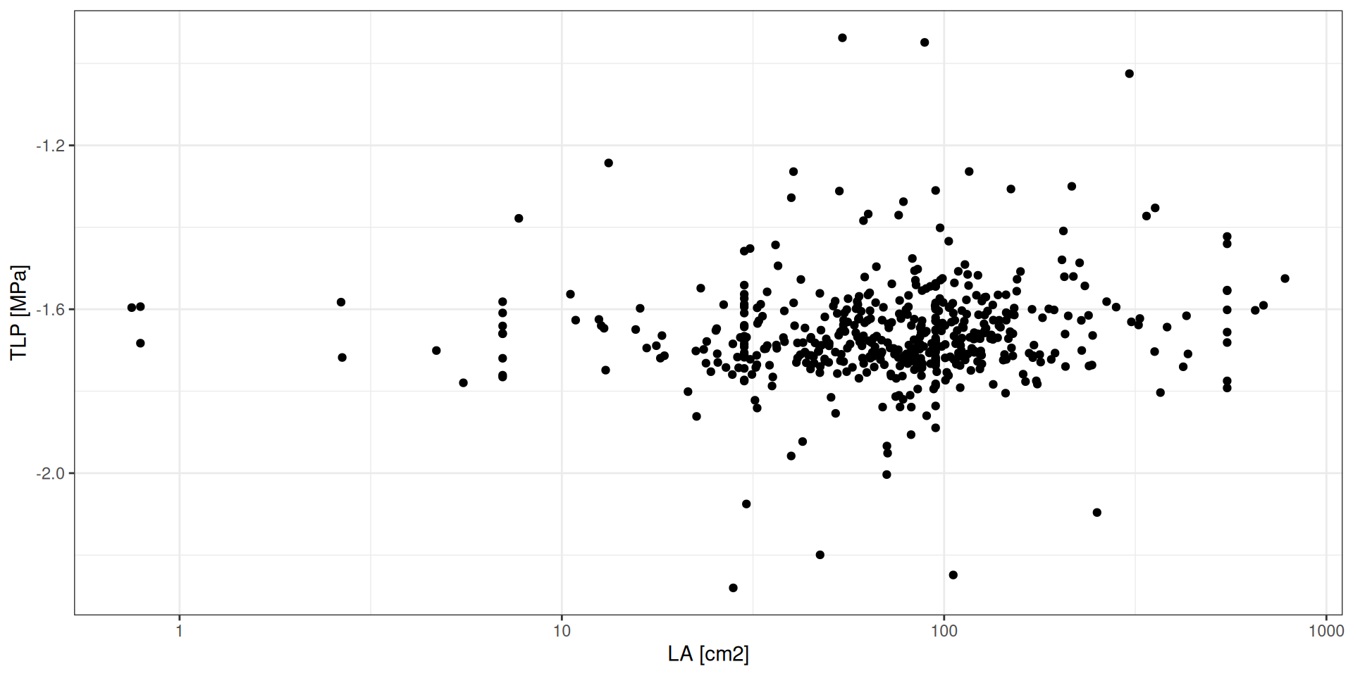
Species
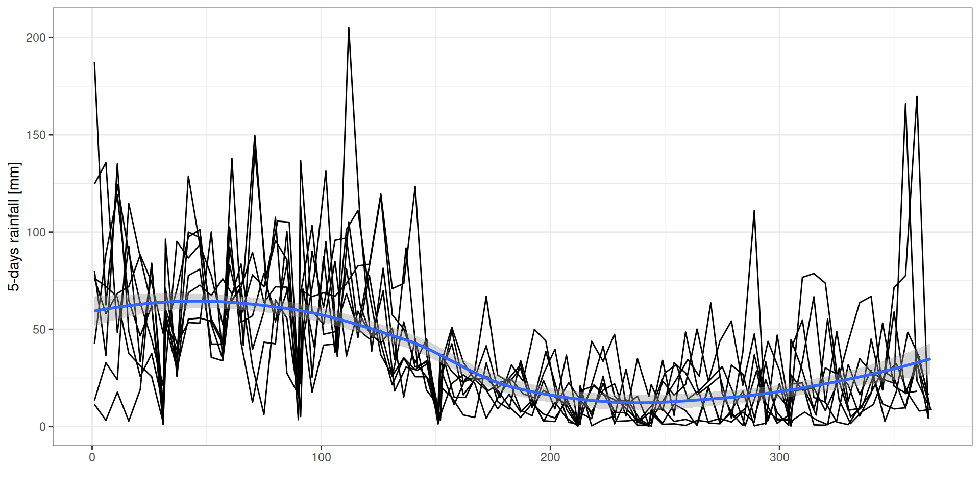
Climate
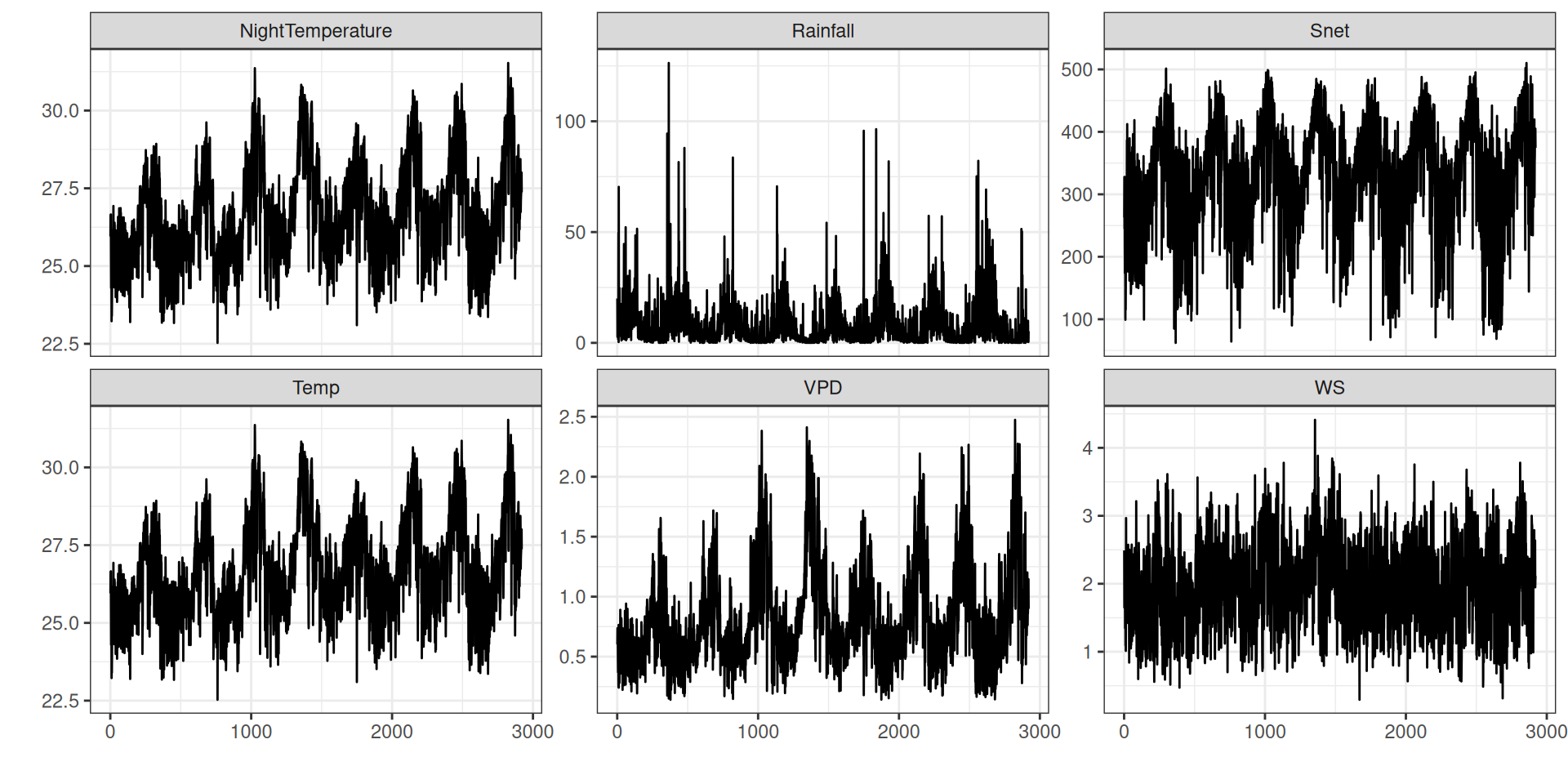
Climate
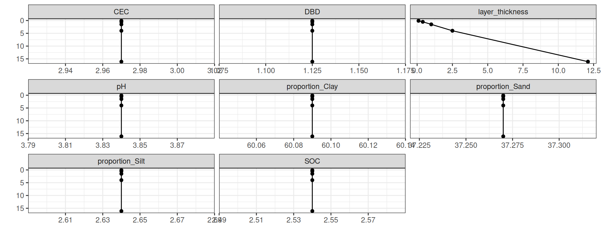
Soil
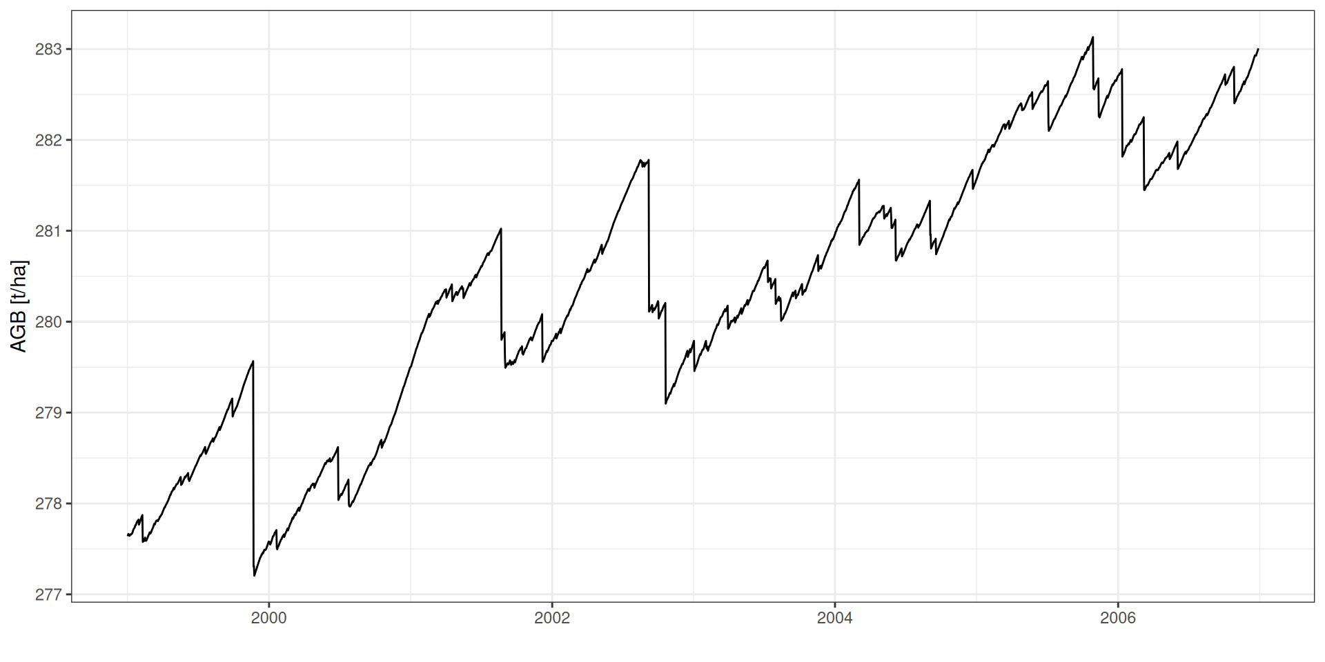
Forest dynamics
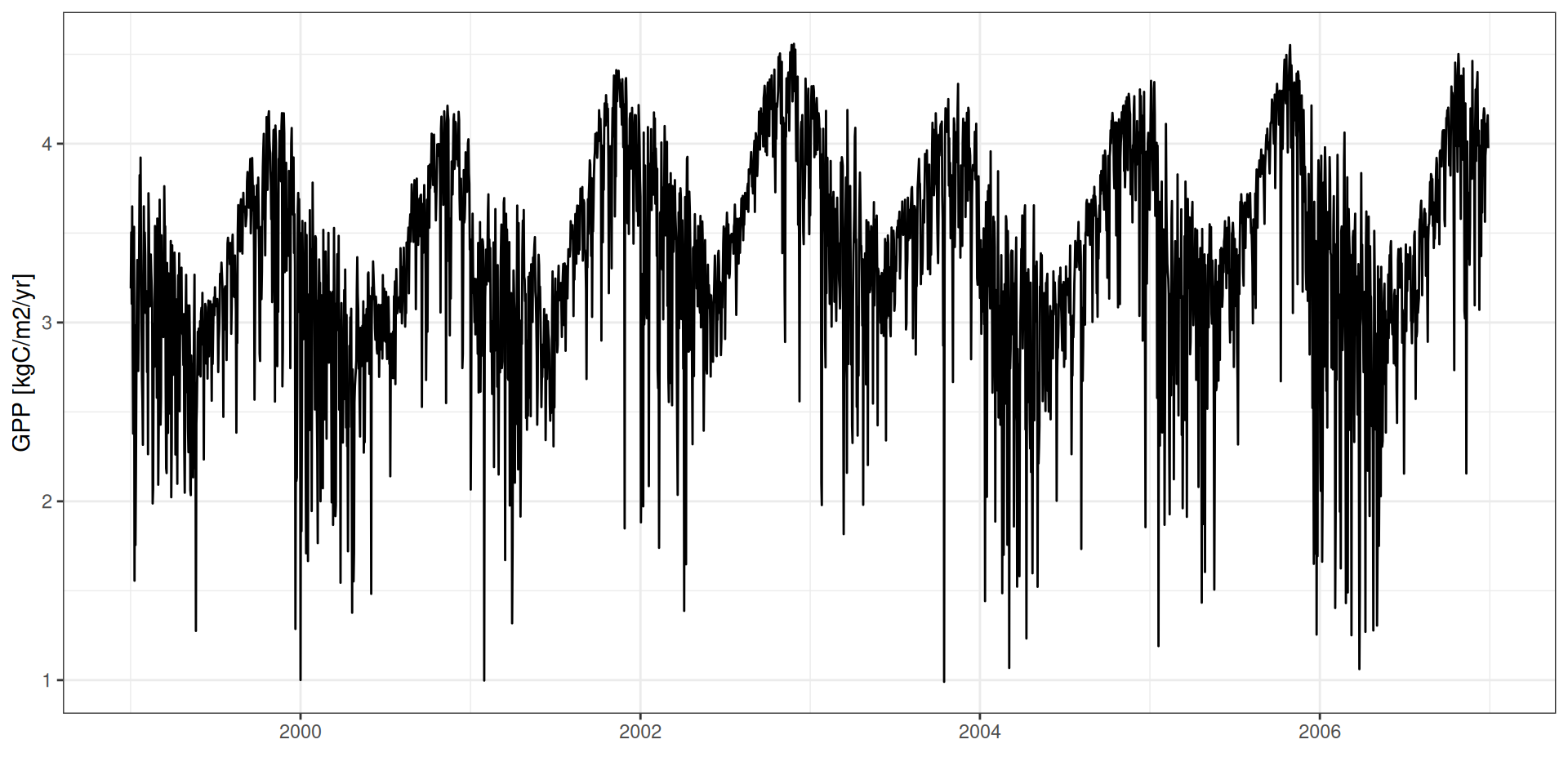
GPP: Gross Primary Productivity
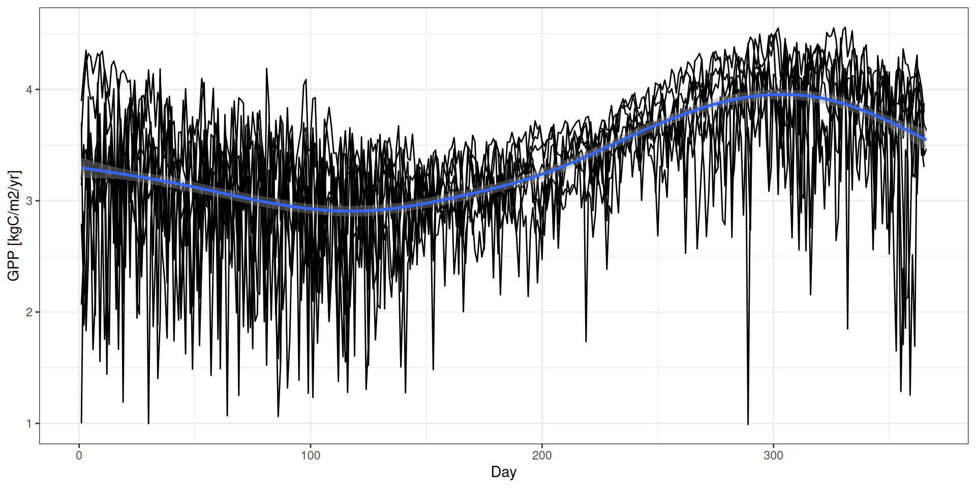
GPP - Seasonality
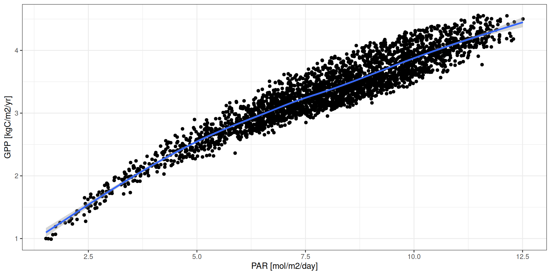
GPP - Drivers
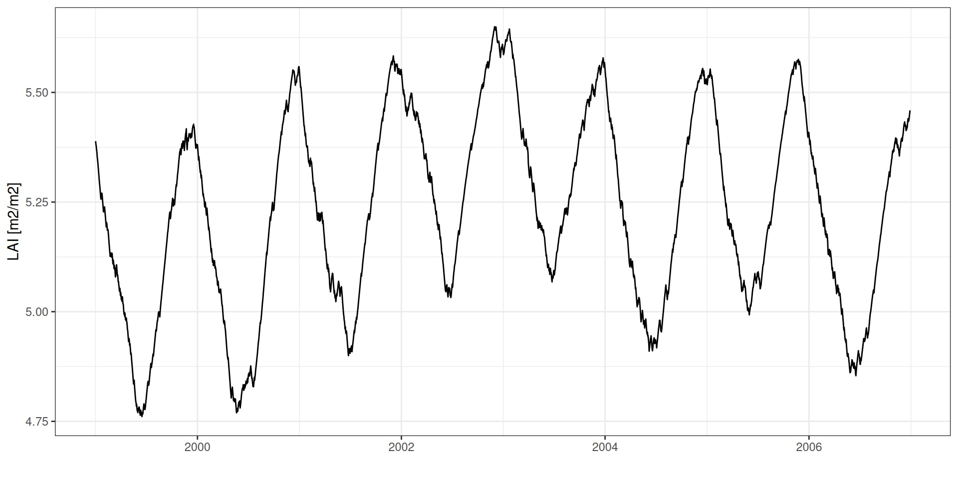
LAI: Leaf Area Index
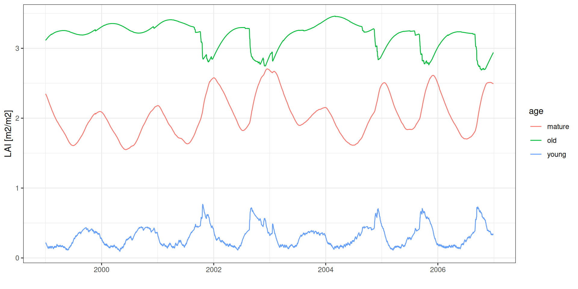
LAI age
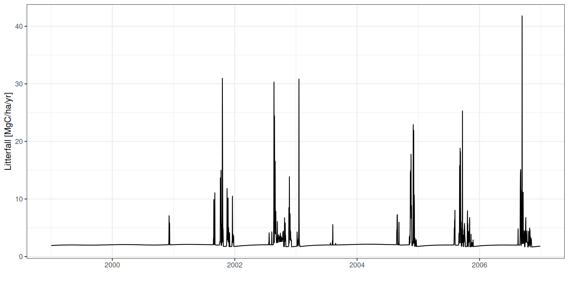
Litterfall
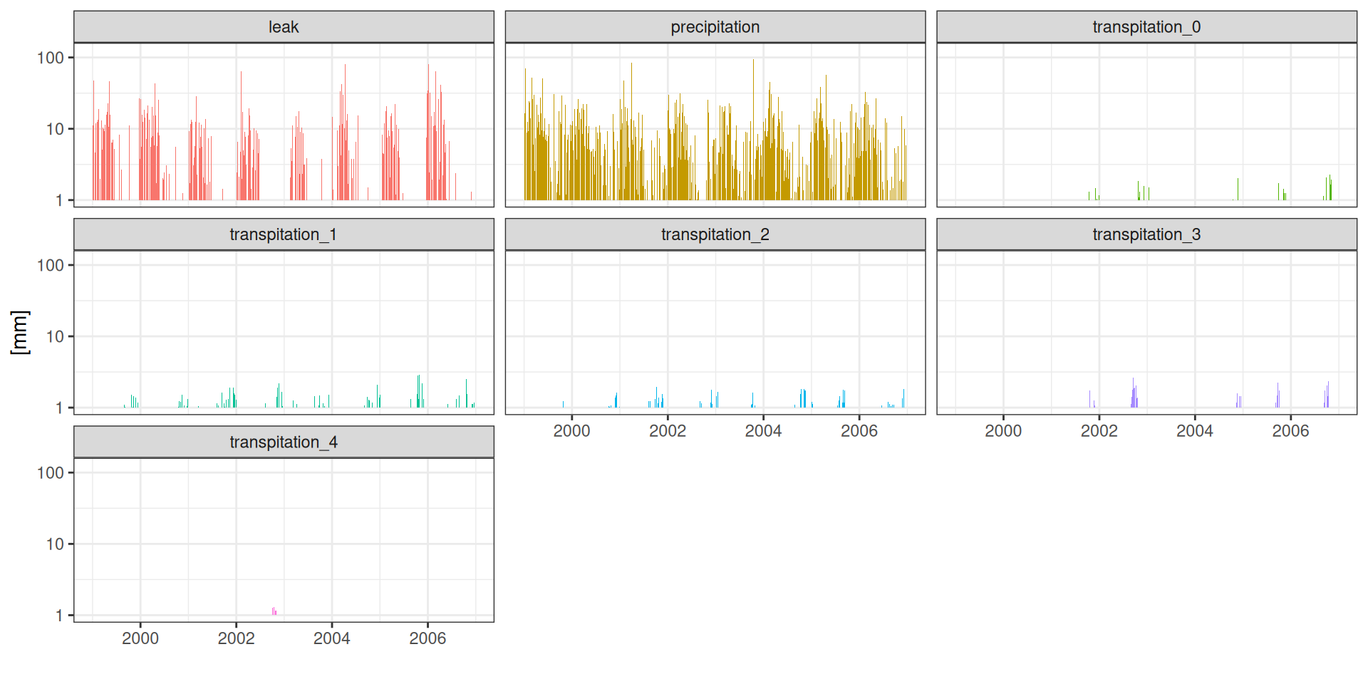
Water balance
Water balance
\[\Delta SWC = P-I-Q-E-T-L\]
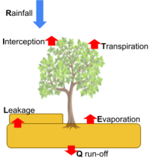
Water balance
Water balance
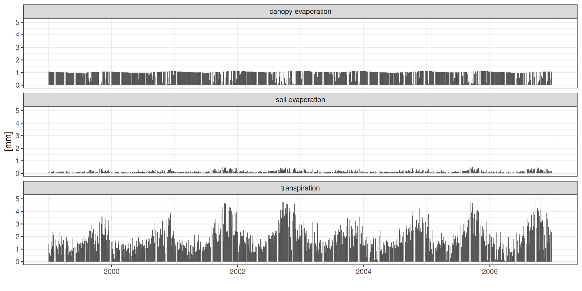
ET : Evapotranspiration
read_tsv("data/day2/R1_0_water_balance.txt") %>%
  mutate(date = as_date("1999-01-01") + iter) %>%
  mutate(et = (transpitation_0 + transpitation_1 + transpitation_2 +
                 transpitation_3 + transpitation_4 + evaporation +
                 (precipitation/1000-throughfall))*1000) %>%
  ggplot(aes(date, et)) +
  geom_line() +   theme_bw() + xlab("") + ylab("ET [mm]")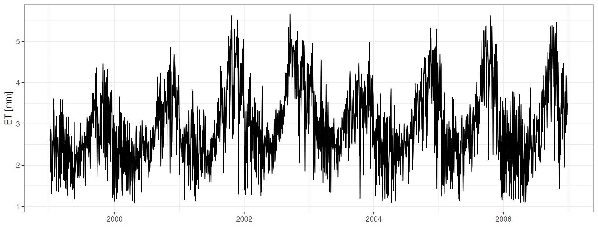
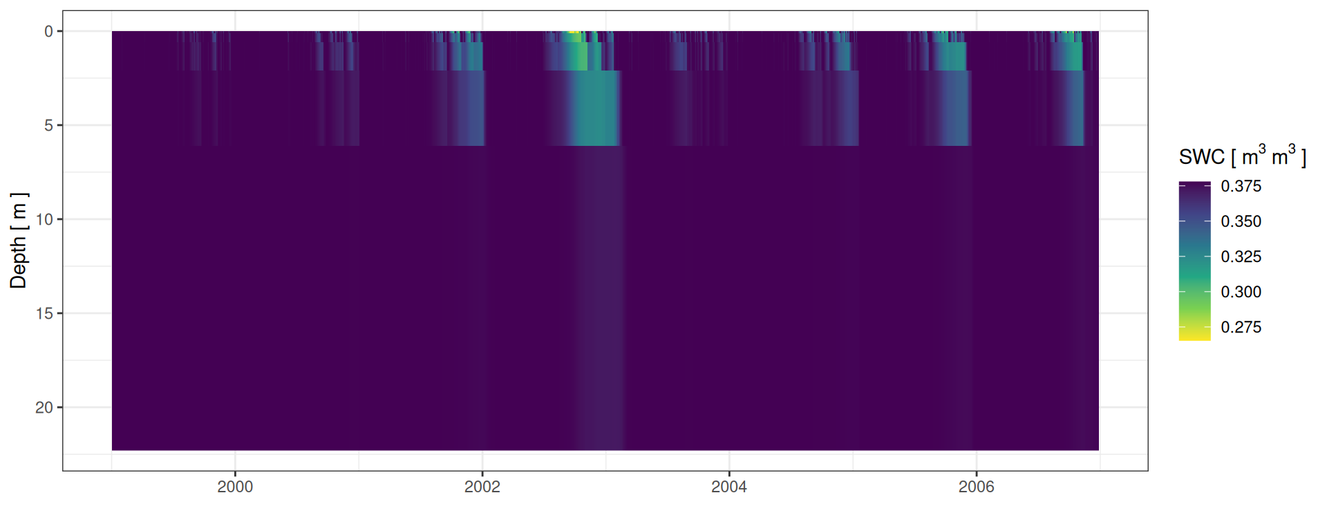
SWC: Soil Water Content
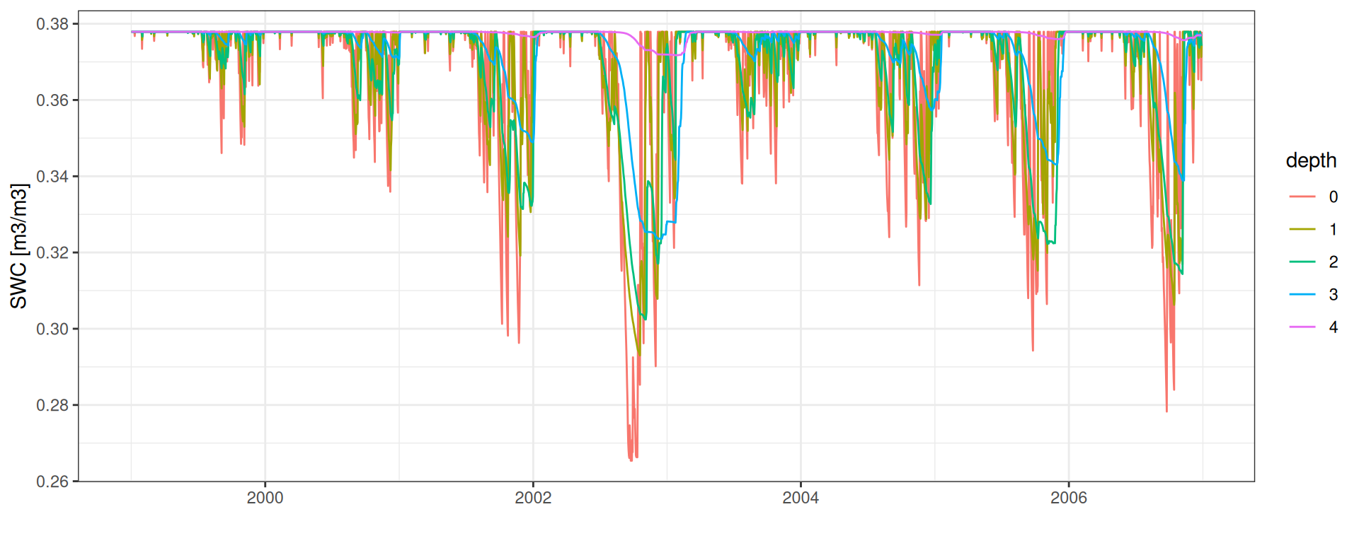
Soil water content
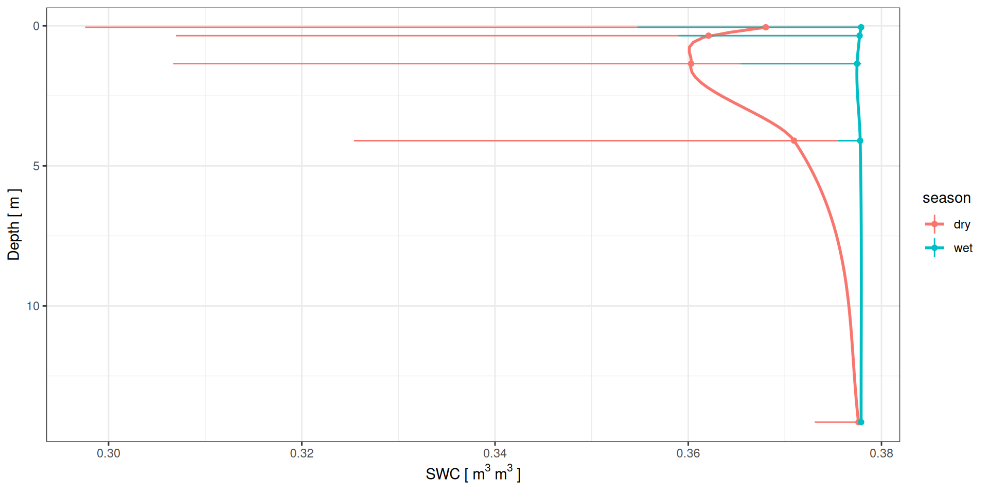
Soil water profiles
References
Maréchaux, Isabelle, Fabian Jörg Fischer, Sylvain Schmitt, and Jérôme Chave. 2025. “TROLL 4.0: Representing Water and Carbon Fluxes, Leaf Phenology, and Intraspecific Trait Variation in a Mixed-Species Individual-Based Forest Dynamics Model Part 1: Model Description.” Geoscientific Model Development 18 (16): 5143–5204. https://doi.org/10.5194/gmd-18-5143-2025.