A simple workflow • rcontroll

This vignette gives a quick example of a simple workflow to produce a single simulation, a stack of simulations, or start from an existing inventory or a previous simulation.

Setup

We will use rcontroll with packages dplyr and tidyr for data wrangling and ggplot2 to do figures.

suppressMessages(library(dplyr))
library(tidyr)
library(ggplot2)
suppressMessages(library(rcontroll))

Data

We load the species data available for French Guiana (TROLLv3_species), with associated climate data (TROLLv3_climatedaytime12) and day variation (TROLLv3_daytimevar). We also load a previous simulation (TROLLv3_output). We generate parameters using generate_parameters for a simulation per month (iterperyear = 12) lasting one year (nbiter = 12) on a 100x100 grid (cols = 100 and rows = 100). We further duplicated parameters with a simulation index using mutate and unnest for a stack of simulations using a seedrain of 5000 (default) and 500 (default/10).

data("TROLLv3_species")
data("TROLLv3_climatedaytime12")
data("TROLLv3_daytimevar")
data("TROLLv3_output")
stack_parameters <- generate_parameters(
  cols = 100, rows = 100,
  iterperyear = 12, nbiter = 12 * 1
) %>%
  mutate(simulation = list(c("seed50000", "seed500"))) %>%
  unnest(simulation)
stack_parameters[62, 2] <- 500 # Cseedrain

Generate parameters

We can generate parameters and view them directly as a table with a description of its effect using generate_parameters and kable.

generate_parameters(cols = 250, rows = 250, nbiter = 12 * 1) %>%
  head() %>%
  knitr::kable()

param	value	description
cols	250	/* nb of columns */
rows	250	/* nb of rows */
HEIGHT	70	/* vertical extent of simulation */
length_dcell	25	/* linear size of a dcell */
nbiter	12	/* total nb of timesteps */
iterperyear	12	/* number of iteration per year */

Simple simulation

We run a simple simulation using the troll function with loaded and generated data. Set verbose to TRUE to see the TROLL log directly in the console.

sim <- troll(
  name = "test",
  global = generate_parameters(
    cols = 100, rows = 100,
    iterperyear = 12, nbiter = 12 * 1
  ),
  species = TROLLv3_species,
  climate = TROLLv3_climatedaytime12,
  daily = TROLLv3_daytimevar,
  verbose = TRUE
)

We can print a simple summary of the simulation.

sim
#> Object of class : trollsim 
#> Name : test 
#> Path :  
#> In memory : TRUE 
#> Extended : TRUE 
#> From data : FALSE 
#> Lidar simulation : FALSE 
#> Random : FALSE 
#> 
#> 2D discrete network: horizontal step =  1 m, one tree per 1 m^2 
#> Number of sites      :  100 x 100 
#> Number of iterations :  12 
#> Duration of timestep :  30.41667 days 
#> Number of Species    :  45

Plot outputs

We can quickly plot simulation outputs using the autoplot method for three types of outputs defined with the what parameter:

the temporal trajectories of variables for the whole ecosystem or user-defined species,
the spatial patterns of variables, including species labels, at forest initial or final pattern,
the distribution of variables at forest initial or final pattern for the whole ecosystem or user-defined species.

For instance here we show species temporal trajectories for all available variables using 4 species: Cecropia obtusa, Dicorynia guianensis, Eperua grandiflora, and Vouacapoua americana:

rcontroll::autoplot(sim,
  what = "temporal",
  species = c(
    "Cecropia_obtusa", "Dicorynia_guianensis",
    "Eperua_grandiflora", "Vouacapoua_americana"
  )
) +
  theme(legend.position = "bottom")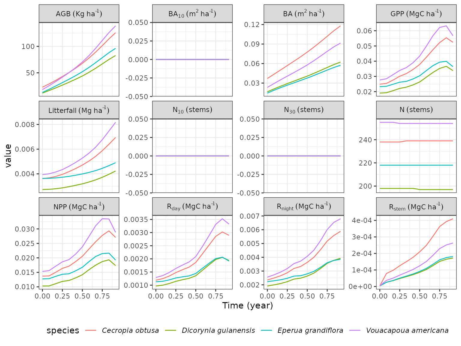

Note that autoplot results in a ggplot2 object that you can modify with the + operator and other ggplot2 commands such as theme used here to change the legend position.

Similarly, we can quickly plot the forest final patterns using autoplot and what defined on spatial:

rcontroll::autoplot(sim, what = "spatial")

Finally, we can quickly plot variables distribution at forest final patterns using autoplot and what defined on distribution:

rcontroll::autoplot(sim,
  what = "distribution",
  variables = c("dbh", "height", "LA", "LMA")
)
#> `stat_bin()` using `bins = 30`. Pick better value with `binwidth`.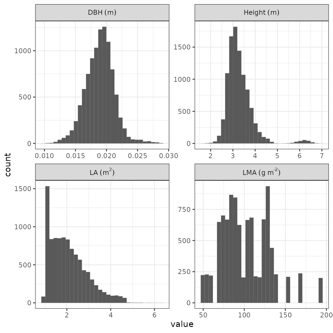

Stack of simulations

We run a stack of simulations using the stack function with loaded and generated data. We can inactivate verbose to see only the loading bar. We can define the number of cores used for parallelization. And we can define a thinning of outputs by giving the number of iterations to be kept to reduce the output size.

sim_stack <- stack(
  name = "teststack",
  simulations = c("seed50000", "seed500"),
  global = stack_parameters,
  species = TROLLv3_species,
  climate = TROLLv3_climatedaytime12,
  daily = TROLLv3_daytimevar,
  verbose = FALSE,
  cores = 2,
  thin = c(1, 5, 10)
)
#>   |                                                                              |                                                                      |   0%  |                                                                              |======================================================================| 100%

We can print a simple summary of the simulations.

sim_stack
#> Object of class : trollstack 
#> Name : teststack 
#> Path :  
#> In memory : TRUE 
#> Number of simulations : 2 
#> Extended : TRUE 
#> From data : FALSE 
#> Lidar simulation : FALSE 
#> Random : FALSE 
#> 
#> 2D discrete network: horizontal step =  1 m, one tree per 1 m^2 
#> Number of sites      :  100 x 100 
#> Number of iterations :  12 
#> Duration of timestep :  30.41667 days 
#> Number of Species    :  45

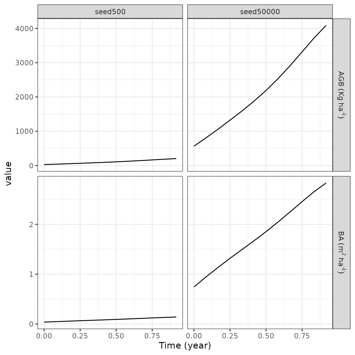
We can quickly plot temporal trajectories for all simulations using autoplot and what defined on temporal, for instance here with basal area (ba) and aboveground biomass (agb):

rcontroll::autoplot(sim_stack,
  what = "temporal",
  variables = c("ba", "agb")
)

Similarly, we can quickly plot the forest final patterns using autoplot and what defined on spatial:

rcontroll::autoplot(sim_stack, what = "spatial")

From a forest

We can also run a simple simulation or a stack of simulations starting from an existing inventory or a previous simulation using the troll function with the forest parameter.

We can first have a look to the ecosystem temporal trajectories of the TROLLv3_output simulation:

rcontroll::autoplot(TROLLv3_output, what = "temporal")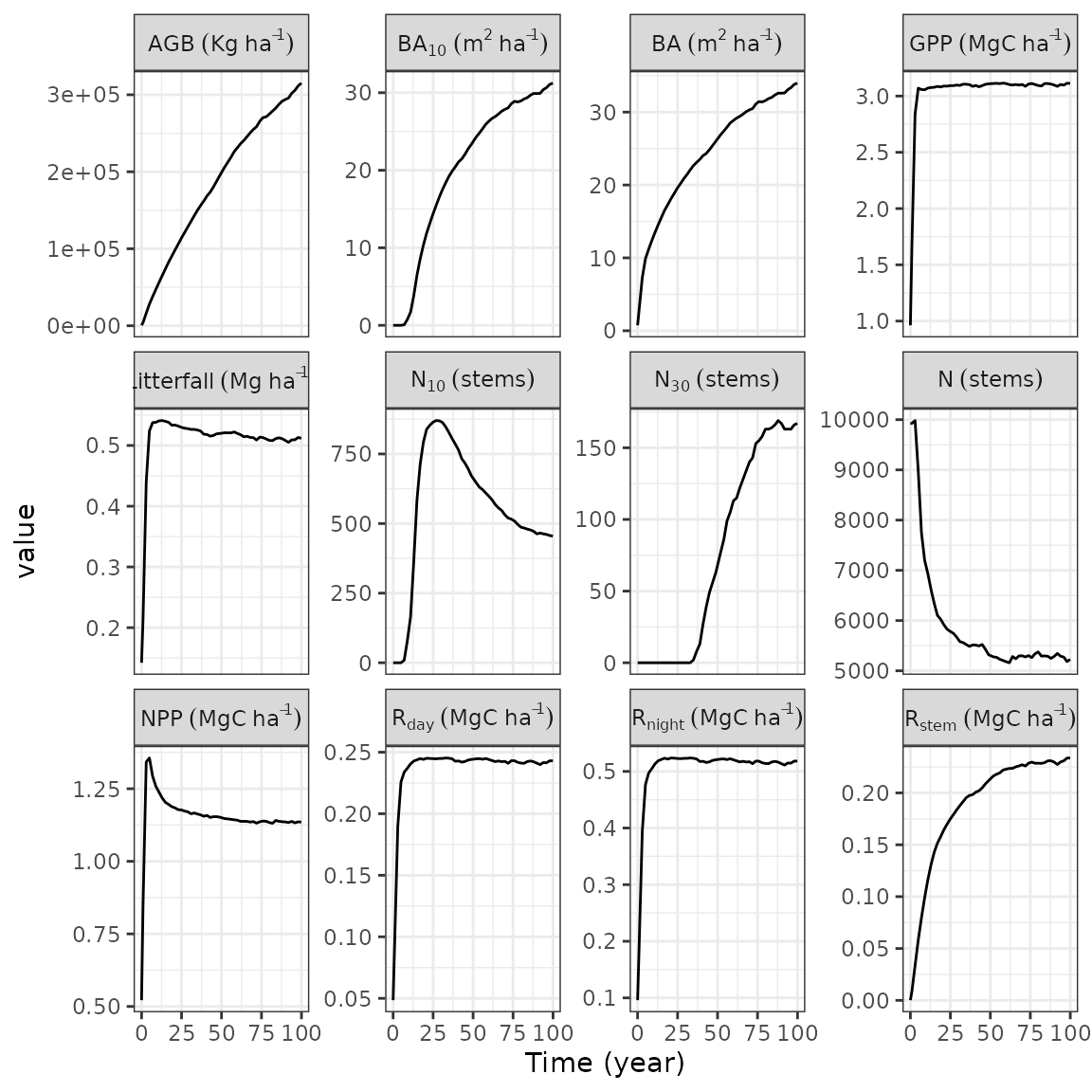

Similarly we can have a look to the the forest final pattern from TROLLv3_output that we will use to initiate the next simulation:

rcontroll::autoplot(TROLLv3_output, what = "spatial", variables = "age")

To run the simulation we first extracted the forest from TROLLv3_output, in which we removed unused columns (not mandatory). Then we extracted the previous simulation parameters to run the new one in similar conditions, we only changed the time length to 12 iterations. And we finally used the same troll function adding the previous forest to initiate the simulation with the forest parameter. A forest inventory can also be used with at least coordinates and DBH.

sim <- troll(
  name = "test",
  global = update_parameters(TROLLv3_output, nbiter = 12 * 1),
  species = TROLLv3_output@inputs$species,
  climate = TROLLv3_output@inputs$climate,
  daily = TROLLv3_output@inputs$daily,
  forest = get_forest(TROLLv3_output),
  verbose = FALSE
)

We can quickly plot temporal trajectories of both simulations to check that the initialization from TROLLv3_output worked. For that we updated the simulation iteration index by adding the number realised in the previous simulation. Then we simply joined ecosystem outputs with bind_rows before using ggplot to show aboveground biomass (agb) temporal trajectory:

sim@ecosystem$iter <- sim@ecosystem$iter + max(TROLLv3_output@ecosystem$iter)
list(
  "TROLLv3_output" = TROLLv3_output@ecosystem,
  "sim" = sim@ecosystem
) %>%
  bind_rows(.id = "simulation") %>%
  ggplot(aes(iter / 12, agb, col = simulation)) +
  geom_point() +
  theme_bw() +
  xlab("Time (years)") +
  ylab(expression(Abovergound ~ biomass ~ (AGB ~ Kg ~ ha^{
    -1
  })))

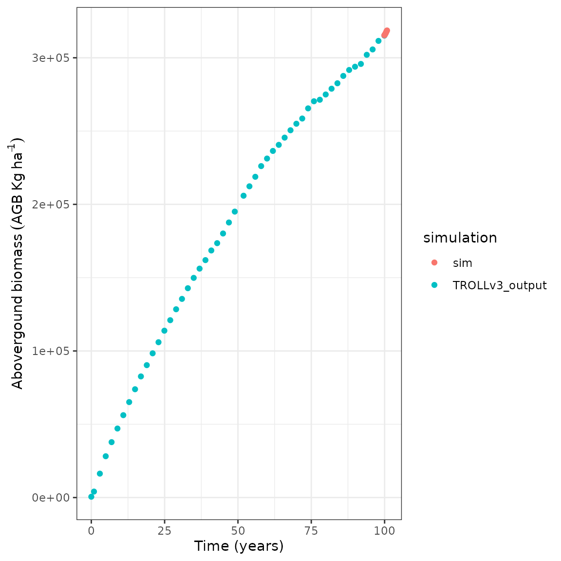
Note how the simulation AGB starts at the end of TROLLv3_output’s temporal trajectory.

Dynamic visualisation

gifs <- autogif(
  name = "dynamic",
  variables = "height_ct",
  global = update_parameters(TROLLv3_output,
    nbiter = 12 * 100,
    extent_visual = 100
  ),
  species = TROLLv3_output@inputs$species,
  climate = TROLLv3_output@inputs$climate,
  daily = TROLLv3_output@inputs$daily,
  forest = get_forest(TROLLv3_output),
  verbose = FALSE
)
gifs$height_ct