Maps

We will collect the following species:

Code

forest %>% 
  group_by(name, code) %>% 
  summarise(N = n()) %>% 
  arrange(desc(N)) %>% 
  knitr::kable()

name	code	N
COPAIBA	COPAI	11
TATAJUBA	TATAJ	11
ANDIROBA	ANDIR	10
ANGELIM VERMELHO	ANGEL	10
ARARAQUANGA	ARARA	10
CASTANHA DO PARA	CASTA	10
CEDRURANA	CEDRU	10
CUMARU	CUMAR	10
CUPIUBA	CUPIU	10
FAVA	FAVA	10
FAVA AMARGA	FAVAA	10
FREIJO	FREIJ	10
JUTAI	JUTAI	10
MARUPA	MARUP	10
MELANCIEIRA	MELAN	10
PARAPARA	PARAP	10
PIQUIA	PIQUI	10
QUARUBA	QUARU	10
TACHI BRANCO	TACHI	10
JARANA	JARAN	9
VIROLA CASCA DE VIDRO	VIROL	9
FAVA ORELHA DE MACACO	FAVAO	6

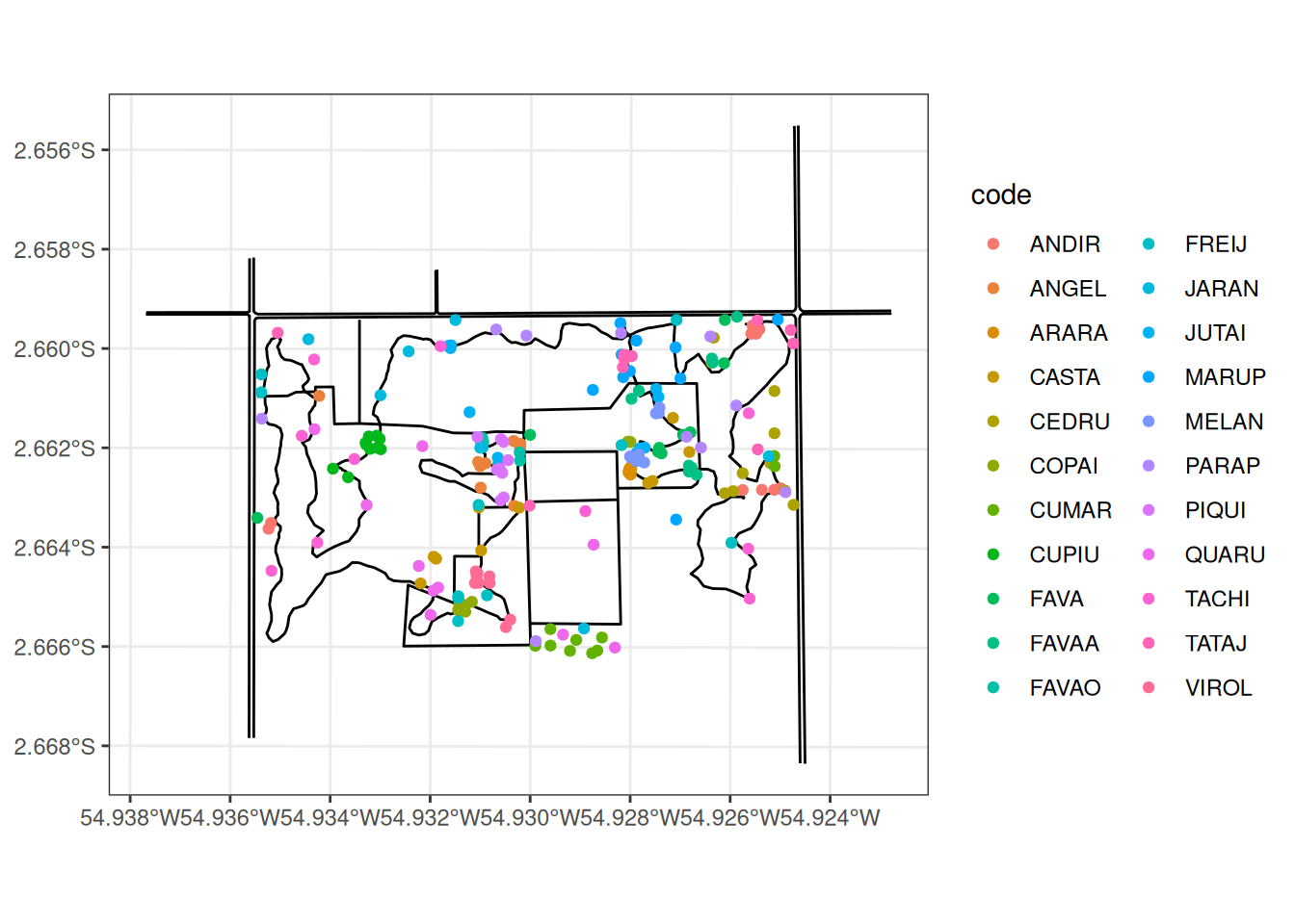
We selected the 10 biggest individuals per species resulting in the following maps of individuals to be collected:

Code

ggplot() +
  geom_sf(data = roads) +
  geom_sf(data = path) +
  geom_sf(data = inventory, aes(col = code)) +
  theme_bw()

Code

g <- ggplot() +
  geom_sf(data = path, col = "darkgrey") +
  geom_sf(data = inventory) +
  ggrepel::geom_text_repel(
      data = inventory,
      aes(label = label, geometry = geometry),
      stat = "sf_coordinates",
      size = 2, max.overlaps = 20) +
  theme_bw() +
  theme(axis.title = element_blank(), axis.text = element_blank(),
        axis.ticks = element_blank(), axis.line = element_blank())
ggsave(g, file = "documents/map.pdf",
       width = 420, height = 297, unit = 'mm', dpi = 300)
knitr::include_graphics("documents/map.pdf")