This book is in Open Review. I want your feedback to make the book better for you and other readers. To add your annotation, select some text and then click the on the pop-up menu. To see the annotations of others, click the in the upper right hand corner of the page

Chapter 5 Other analyses

In this chapter, I quickly investigated effects of functional traits and weather on individual growth.

5.1 Methods

I used linear model for individual growth potential relation to functional traits at the individual or species level. For each dataset, I first used a step procedure to select explanatory variables before using linear models with multiple variables. I then plotted the individual relations between response and explanatory variables.

5.2 Results

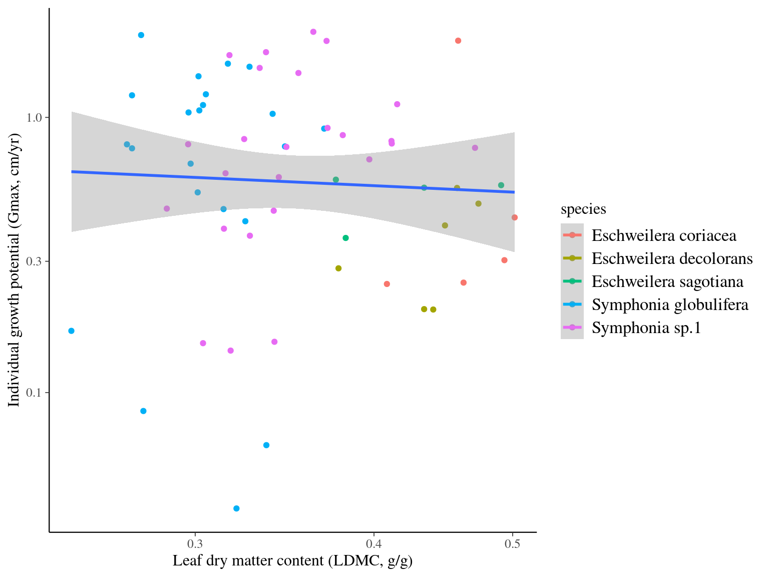
5.2.1 ParacouITV

Interestingly, leaf dry matter content seems to drive individual growth potential within species of Symphonia and Eschweilera genera (\(\beta=-0.91, p=0.016, R^2=0.083\)), but the signal is weak.

	log(gmax)
Predictors	Estimates	CI	p
(Intercept)	-1.65	-4.82 – 1.52	0.302
CC	0.02	-0.00 – 0.04	0.090
LA [log]	-0.14	-0.50 – 0.22	0.430
LDMC [log]	-0.41	-1.80 – 0.97	0.553
Observations	62
R² / R² adjusted	0.089 / 0.042

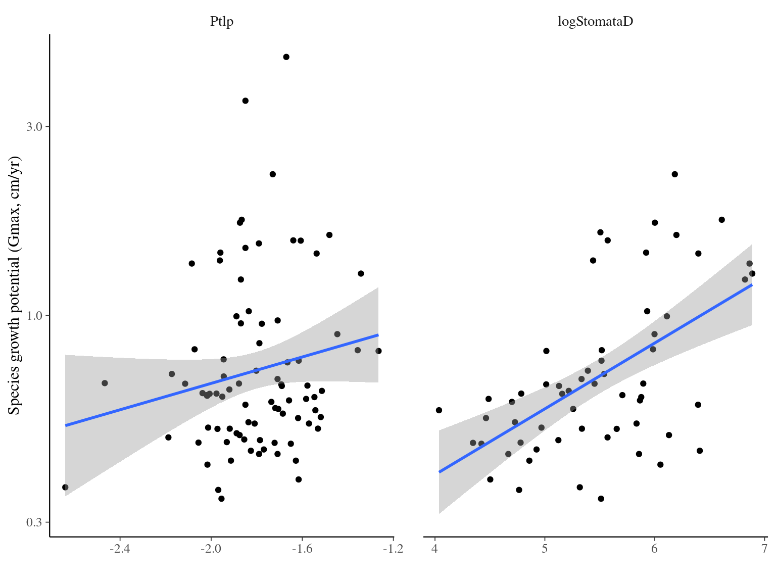
5.2.2 hydroParacou

Interestingly, turgor loss point and stomatal density appear to influence species growth potential with a positive effect (\(\beta=1.13, p=0.004\) & \(\beta=0.28, p<0.001\), \(R^2=0.0312\)). Species with more stomata lose their turgidity more quickly but grow faster.

	log(gmax)
Predictors	Estimates	CI	p
(Intercept)	0.48	-0.25 – 1.22	0.192
Ptlp	0.76	0.03 – 1.48	0.042
CN [log]	-0.40	-0.81 – 0.01	0.058
stomataD [log]	0.34	0.19 – 0.49	<0.001
Observations	58
R² / R² adjusted	0.427 / 0.395

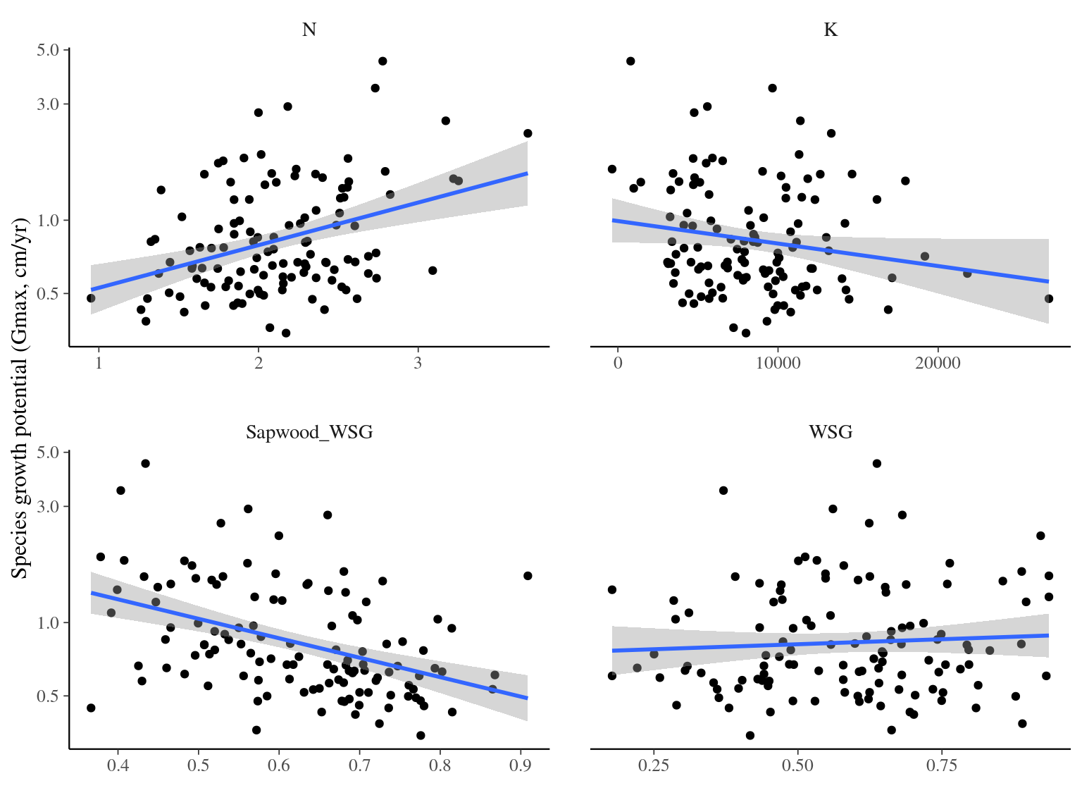
5.2.3 Vleminckx et al. 2021

	log(gmax)
Predictors	Estimates	CI	p
(Intercept)	-0.19	-0.26 – -0.12	<0.001
C	-0.05	-0.13 – 0.03	0.210
N	0.20	0.12 – 0.28	<0.001
K	-0.15	-0.23 – -0.07	<0.001
Sapwood WSG	-0.23	-0.31 – -0.15	<0.001
WSG	0.10	0.02 – 0.18	0.015
Observations	120
R² / R² adjusted	0.397 / 0.371

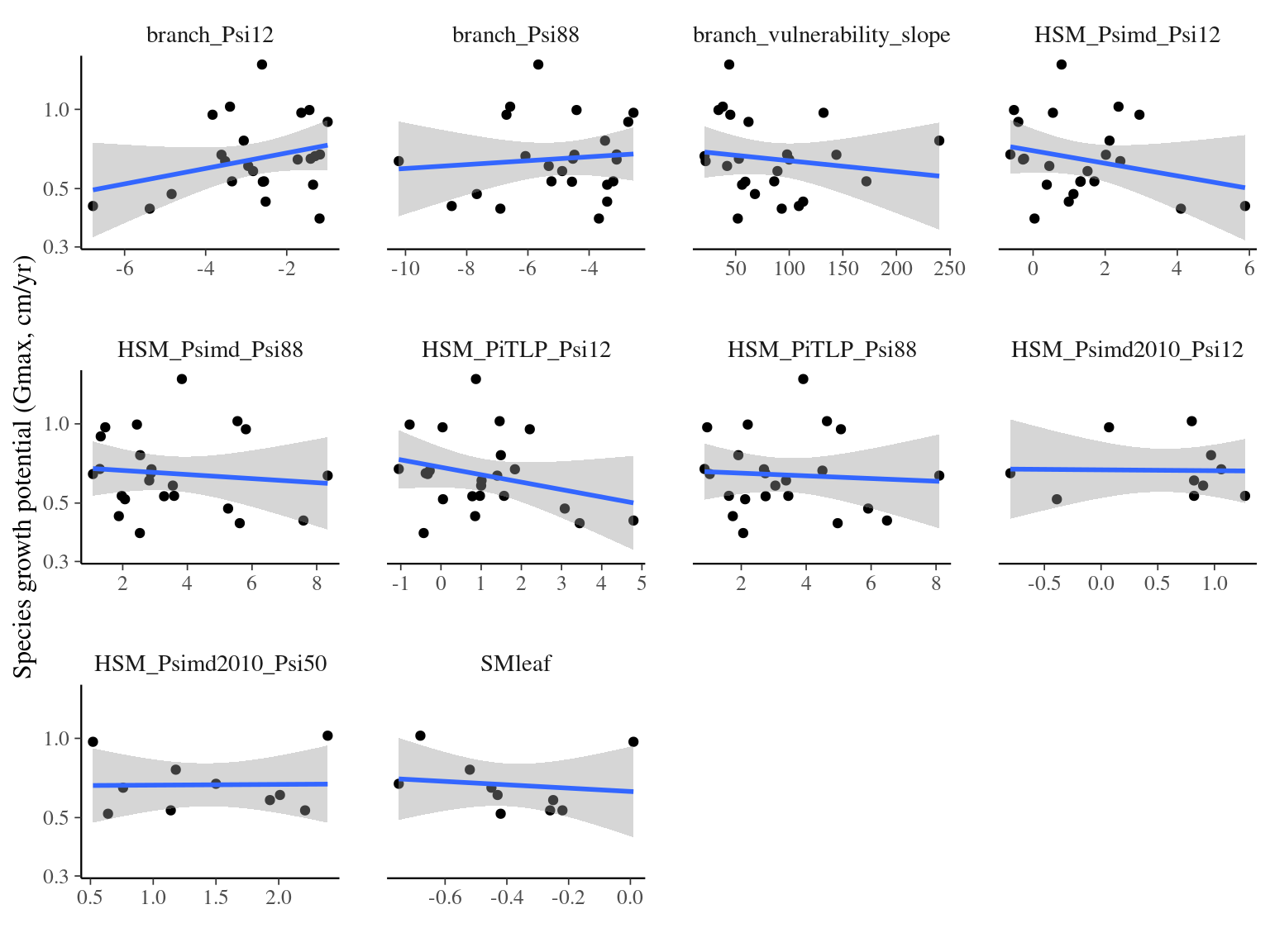
5.2.4 Ziegler et al. 2019

	log(gmax)
Predictors	Estimates	CI	p
(Intercept)	-0.25	-0.75 – 0.25	0.310
branch vulnerability slope	-0.00	-0.00 – 0.00	0.419
HSM PiTLP Psi88	-0.03	-0.12 – 0.06	0.536
Observations	23
R² / R² adjusted	0.037 / -0.059

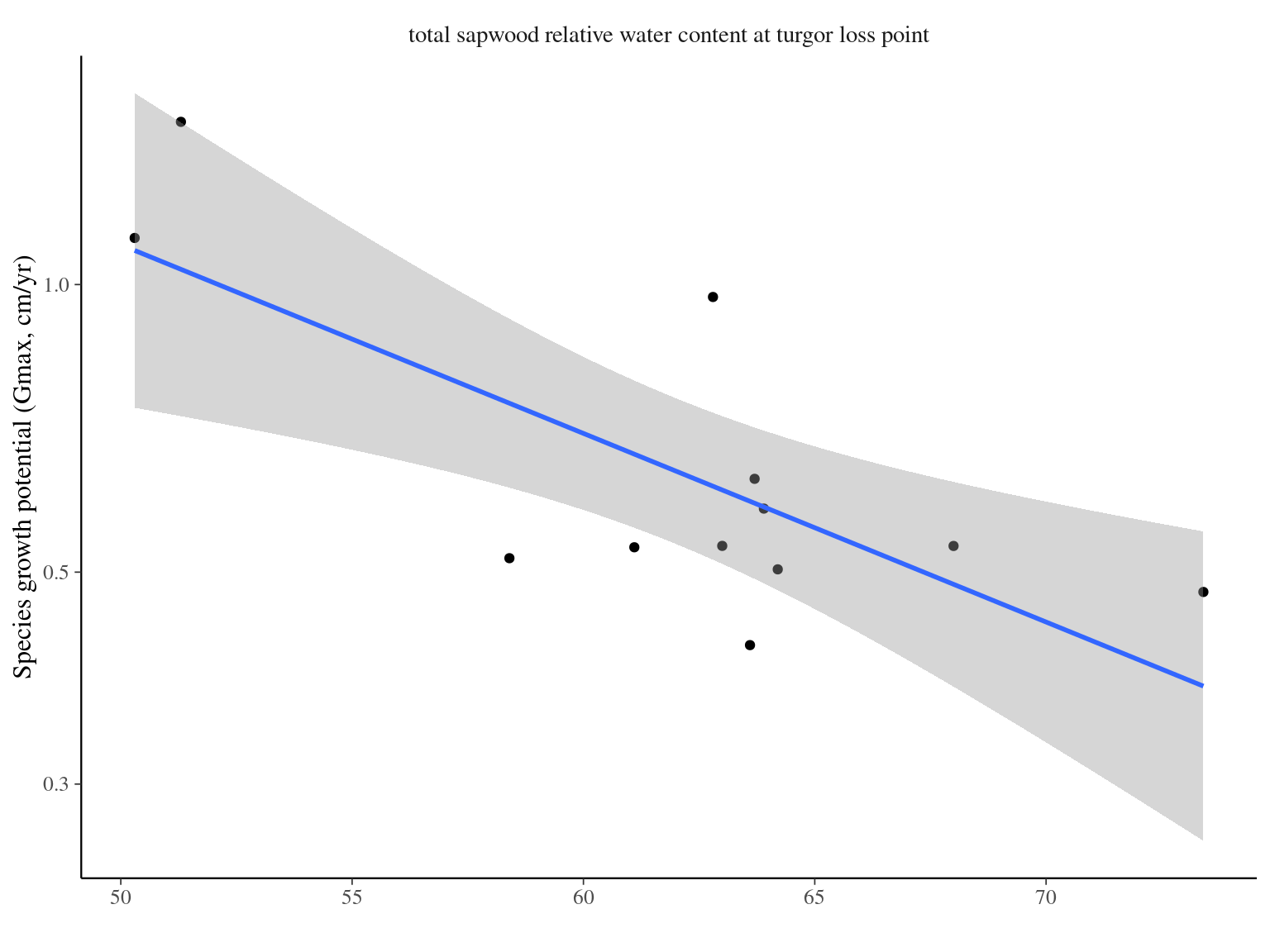
5.2.5 Santiago et al. 2018

	log(gmax)
Predictors	Estimates	CI	p
(Intercept)	2.37	0.58 – 4.16	0.015
total sapwood relative water content at turgor loss point	-0.05	-0.07 – -0.02	0.006
Observations	12
R² / R² adjusted	0.553 / 0.508

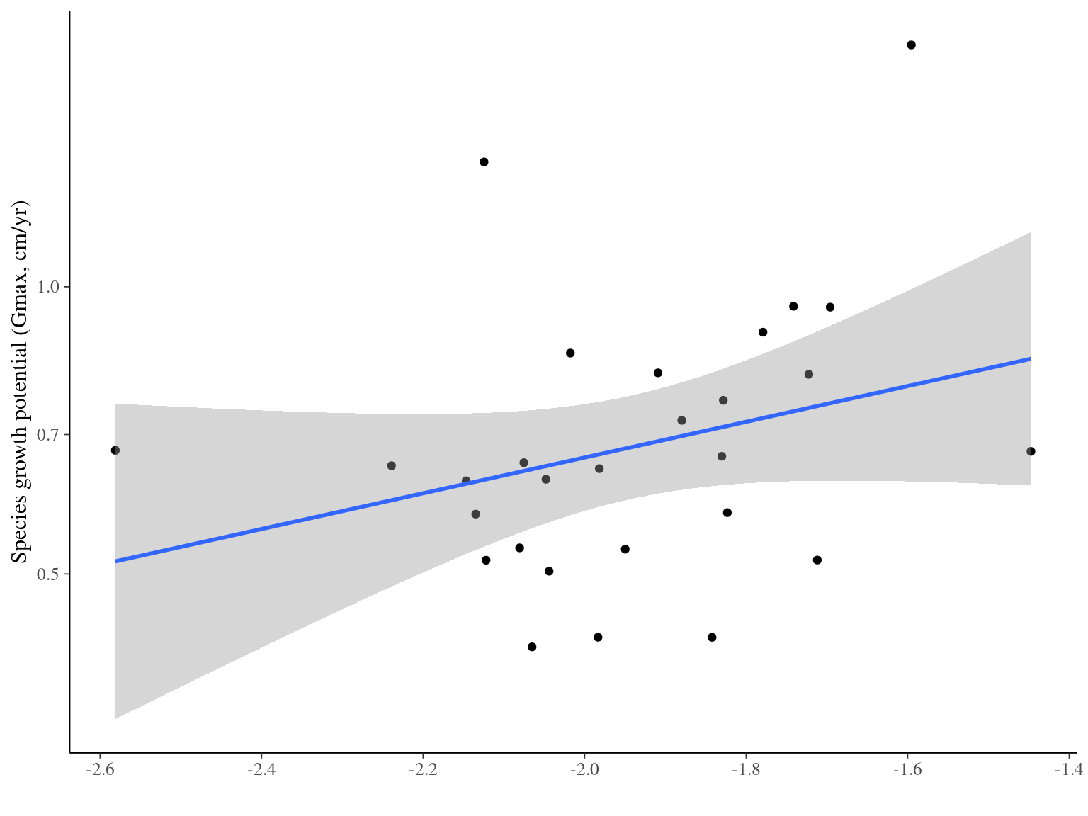
5.2.6 Maréchaux et al. 2015

	log(gmax)
Predictors	Estimates	CI	p
(Intercept)	0.45	-0.65 – 1.55	0.409
Pi tlp	0.43	-0.13 – 0.99	0.128
Observations	28
R² / R² adjusted	0.087 / 0.052

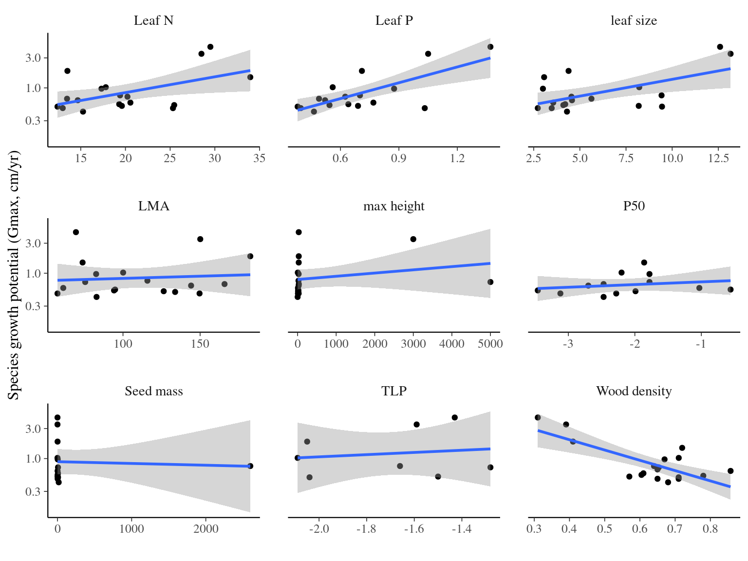
5.2.7 Guillemot et al. 2022

	log(gmax)
Predictors	Estimates	CI	p
(Intercept)	0.24	-1.84 – 2.33	0.804
leaf size [log]	0.07	-0.01 – 0.15	0.101
Leaf N	-0.02	-0.09 – 0.05	0.551
Leaf P	1.15	-0.55 – 2.85	0.165
Wood density	-2.05	-4.40 – 0.29	0.080
Observations	17
R² / R² adjusted	0.773 / 0.698