Chapter 2 Design of probes set
The genomic and transcriptomic resources used for the design were comprised of a published low-coverage draft genome from Africa (Olsson et al. 2017), an unpublished draft genome from French Guiana [Scotti et al., in prep], an unpublished transcriptome from 20 juveniles from French Guiana [Tysklind et al., in prep], and reduced-representation genomic sequence reads of individuals from French Guiana [Torroba-Balmori et al., unpublished].
We aligned genomic reads on the two genome drafts with bwa (Li & Durbin 2009).
We kept scaffolds from the two genome drafts with a length of more than 1 kbp and at least one matching alignment with a read with a single match on the genome, and merged the two filtered genome drafts with quickmerge (Chakraborty et al. 2016).
We aligned transcripts on the new filtered genome draft with BLAT (Kent 2002) and selected 533 scaffolds without transcript-match, i.e. anonymous scaffolds.
We masked repetitive regions with RepeatMasker (Smit et al. 2015) and selected 533 1-kbp anonymous loci within the 533 previous scaffolds.
Similarly, we filtered transcripts from the 20 juveniles of Symphonia globulifera from French Guiana [Tysklind et al., in prep] based on SNP quality, type and frequency.
We further detected open reading frames (ORFs) using transdecoder (Haas et al. 2013),
and selected transcripts with non-overlapping ORFs including a start codon.
We kept ORFs with an alignment on scaffolds from the aforementioned genome draft for Symphonia using BLAT (Kent 2002),
and masked repetitive regions with RepeatMasker (Smit et al. 2015).
We selected 1,150 genic loci of 500-bp to 1-kbp, from 100 bp before the start to a maximum of 900 bp after the end of the ORFs, resulting in 1-Mbp genomic loci that included a coding region.
2.1 Scotti et al. (in prep) scaffolds preparation
2.1.1 Filtering scaffolds over \(1kbp\)
We first filtered scaffolds with a width of more than 1000 bp.
2.1.2 Renaming
For all scaffolds we used the following code : **Ivan_2018_[file name without .scafSeq]_[scaffold name]**.
dir.create(file.path(path, "Ivan_2018", "renamed_scf_1000"))
files <- list.files(file.path(path, "Ivan_2018", "scf_1000"))
sapply(files, function(file){
  scf <- readDNAStringSet(file.path(path, "Ivan_2018", "scf_1000", file))
  names(scf) <- paste0("Ivan_2018_", gsub(".scafSeq", "", file), "_", gsub(" ", "_", names(scf)))
  writeXStringSet(scf, file.path(path, "Ivan_2018", "renamed_scf_1000",
                                 paste0(gsub(".scafSeq", "", file), ".1000.renamed.scafSeq")))
}, simplify = F)
unlink(file.path(path, "Ivan_2018", "scf_1000"), recursive = T)
2.1.3 Libraries merging
We successively merged scaffolds from 6 libraries with quickmerge.
cd ~/Documents/BIOGECO/PhD/data/Symphonia_Genomes/Ivan_2018/renamed_scf_1000
ref=(sympho47_1L1_002.1000.renamed.scafSeq merge1.fasta merge2.fasta merge3.fasta merge4.fasta merge5.fasta merge6.fasta merge7.fasta)
query=(sympho47_1L2_001.1000.renamed.scafSeq sympho47_2L1_008.1000.renamed.scafSeq sympho47_2L1_009.1000.renamed.scafSeq sympho47_2L1_010.1000.renamed.scafSeq sympho47_2L1_011.1000.renamed.scafSeq sympho47_2L1_012.1000.renamed.scafSeq sympho47_3L2_013.1000.renamed.scafSeq sympho47_4L1_014.1000.renamed.scafSeq)
for i in {0..7}
do
  mkdir merge$i
  cp  "${ref[$i]}" "${query[$i]}" ./merge$i/
  cd merge$i
  nucmer -l 100 -prefix out ${ref[$i]} ${query[$i]}
  delta-filter -i 95 -r -q out.delta > out.rq.delta
  ~/Tools/quickmerge/quickmerge -d out.rq.delta -q ${query[$i]} -r ${ref[$i]} -hco 5.0 -c 1.5 -l n -ml m
  cd ..
  cp merge$i/merged.fasta ./merge$((i+1)).fasta
done2.1.4 Removing scaffolds with multimatch blasted consensus sequence from Torroba-Balmori et al. (unpublished)
We used the consensus sequence for French Guianan reads from Torroba-Balmori et al. (unpublished) previously assembled with ipyrad.
We kept the first sequence of the consensus loci file and recoded it to fasta (see loci2fa.py script below).
We then blasted the consensus sequences on merged scaffolds from Scotti et al (in prep) with blastn in order to detect scaffolds with repetitive regions (multi-mapped consensus sequences).
Repetitive sequences have been saved as a list and removed to generate the final list of selected scaffolds.
infile = open("symphoGbS2.loci", "r")
outfile = open("symphoGbS2.firstline.fasta", "w")
loci = infile.read().split("|\n")[:-1]
for loc in loci:
    reads = loc.split("\n")
    name, seq = reads[0].split()
    print >>outfile, ">"+name+"\n"+seq
outfile.close()
cd ~/Documents/BIOGECO/PhD/data/Symphonia_Torroba/assembly/symphoGbS2_outfile
python loci2fa.py
cat symphoGbS2.firstline.fasta | tr - N >> symphoGbS2.firstline.fastacd ~/Documents/BIOGECO/PhD/data/Symphonia_Genomes/Ivan_2018
query=~/Documents/BIOGECO/PhD/data/Symphonia_Torroba/assembly/symphoGbS2_outfiles/symphoGbS2.firstline.fasta
blastn -db merged_1000/merged_1000.fa -query $query -out blast_consensus_torroba2.txt -evalue 1e-10 -best_hit_score_edge 0.05 -best_hit_overhang 0.25 -outfmt 6 -perc_identity 75 -max_target_seqs 10blast <- read_tsv(file.path(path, "Ivan_2018", "torroba_blast",
"blast_consensus_torroba2.txt"), col_names = F)
names(blast) <- c("Read", "Scaffold", "Perc_Ident", "Alignment_length", "Mismatches",
"Gap_openings", "R_start", "R_end", "S_start", "S_end", "E", "Bits")
write_file(paste(unique(blast$Scaffold), collapse = "\n"),
file.path(path, "Ivan_2018", "torroba_blast",
"selected_scaffolds_blast_consensus2.list"))seqtk subseq merged_1000/merged_1000.fa selected_scaffolds_blast_consensus2.list >> selected_scaffolds_blast_consensus2.faIn total 542 scaffolds from Scotti et al (in prep) matched consensus sequences from Torroba-Balmori et al. (unpublished). Several scaffolds obtained multiple matches that we cannot use for probes. We thus excluded the whole scaffold if the scaffold is shorter than 2000 bp, or the scaffold region matching the raw read if the scaffold is longer than 2000 bp.
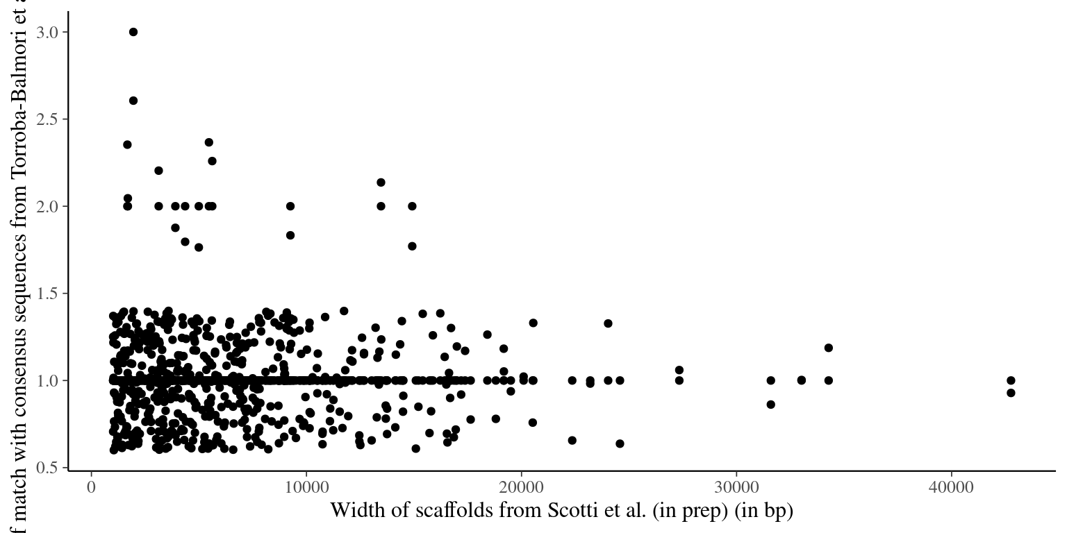
Figure 2.1: Number of match with Torroba consensus reads vs gene width.
| Scaffold | width | remove | cut |
|---|---|---|---|
| Ivan_2018_sympho47_2L1_012_scaffold197676__8.6 | 4993 | 4993-4932 | |
| Ivan_2018_sympho47_2L1_012_scaffold246452__6.6 | 3103 | 2980-3058 | |
| Ivan_2018_sympho47_2L1_012_scaffold26367__7.7 | 2168 | 2118-2168 | |
| Ivan_2018_sympho47_2L1_012_scaffold463128__4.7 | 2188 | 667-586 | |
| Ivan_2018_sympho47_2L1_008_scaffold309475__2.1 | 3525 | 342-292 |
The following scaffolds have been removed due to multiple matches and a length \(<200bp\): 2L1_012_scaffold645876__7.5, 2L1_012_scaffold176548__7.1, 2L1_012_scaffold21882__4.9, 2L1_012_scaffold9236__6.0. The others have been cut (see table 2.1).
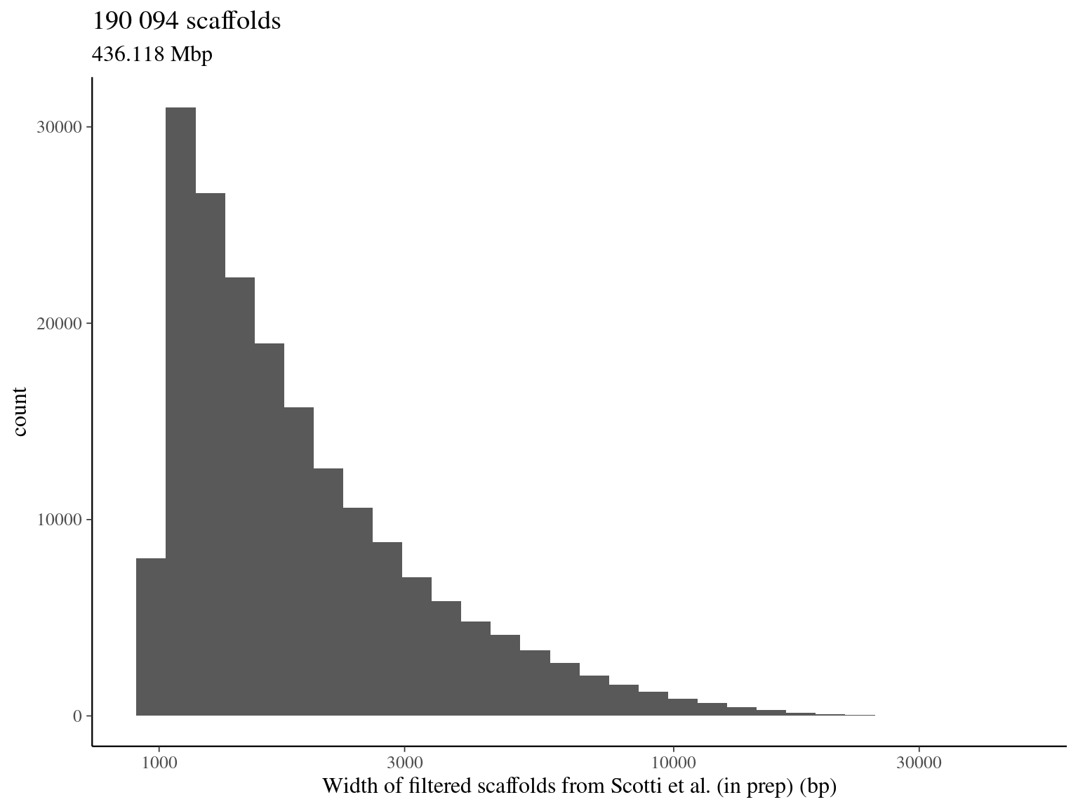
2.1.5 Total filtered scaffolds
2.2 Olsson et al. (2017) scaffolds preparation
African genome from Olsson et al. (2017).
2.2.1 Renaming
We renamed scaffolds from Olsson using the following code : Olsson_2017_[scaffold name].
2.2.2 Removing scaffolds with multimatch blasted consensus sequence from Torroba-Balmori et al. (unpublished)
We used the consensus sequence for French Guianan reads from Torroba-Balmori et al. (unpublished), by blasting them on scaffolds from Olsson et al. (2017) with blastn.
cd ~/Documents/BIOGECO/PhD/data/Symphonia_Genomes/Olsson_2016
cd Olsson2017
makeblastdb -in Olsson2017.fa -parse_seqids -dbtype nucl
cd ..
query=~/Documents/BIOGECO/PhD/data/Symphonia_Torroba/assembly/symphoGbS2_outfiles/symphoGbS2.firstline.fasta
blastn -db Olsson2017/Olsson2017.fa -query $query -out blast_consensus_torroba2.txt -evalue 1e-10 -best_hit_score_edge 0.05 -best_hit_overhang 0.25 -outfmt 6 -perc_identity 75 -max_target_seqs 10
blast <- read_tsv(file.path(path, "Olsson_2016", "torroba_blast",
"blast_consensus_torroba2.txt"), col_names = F)
names(blast) <- c("Read", "Scaffold", "Perc_Ident", "Alignment_length", "Mismatches",
"Gap_openings", "R_start", "R_end", "S_start", "S_end", "E", "Bits")
write_file(paste(unique(blast$Scaffold), collapse = "\n"),
file.path(path, "Olsson_2016", "torroba_blast",
"selected_scaffolds_blast_consensus2.list"))seqtk subseq Olsson2017/Olsson2017.fa selected_scaffolds_blast_consensus2.list >> selected_scaffolds_blast_consensus2.faWe obtained most scaffolds with a single match including a broad range of sizes (from 100 bp to 33.2 kbp). In total 688 scaffolds from Olsson et al. (2017) match consensus sequences from Torroba-Balmori et al. (unpublished). Several scaffolds obtained multiple matches that we cannot use for probes. We thus excluded the whole scaffold if the scaffold is shorter than 2000 bp, or the scaffold region matching the raw read if the scaffold is longer than 2000 bp.
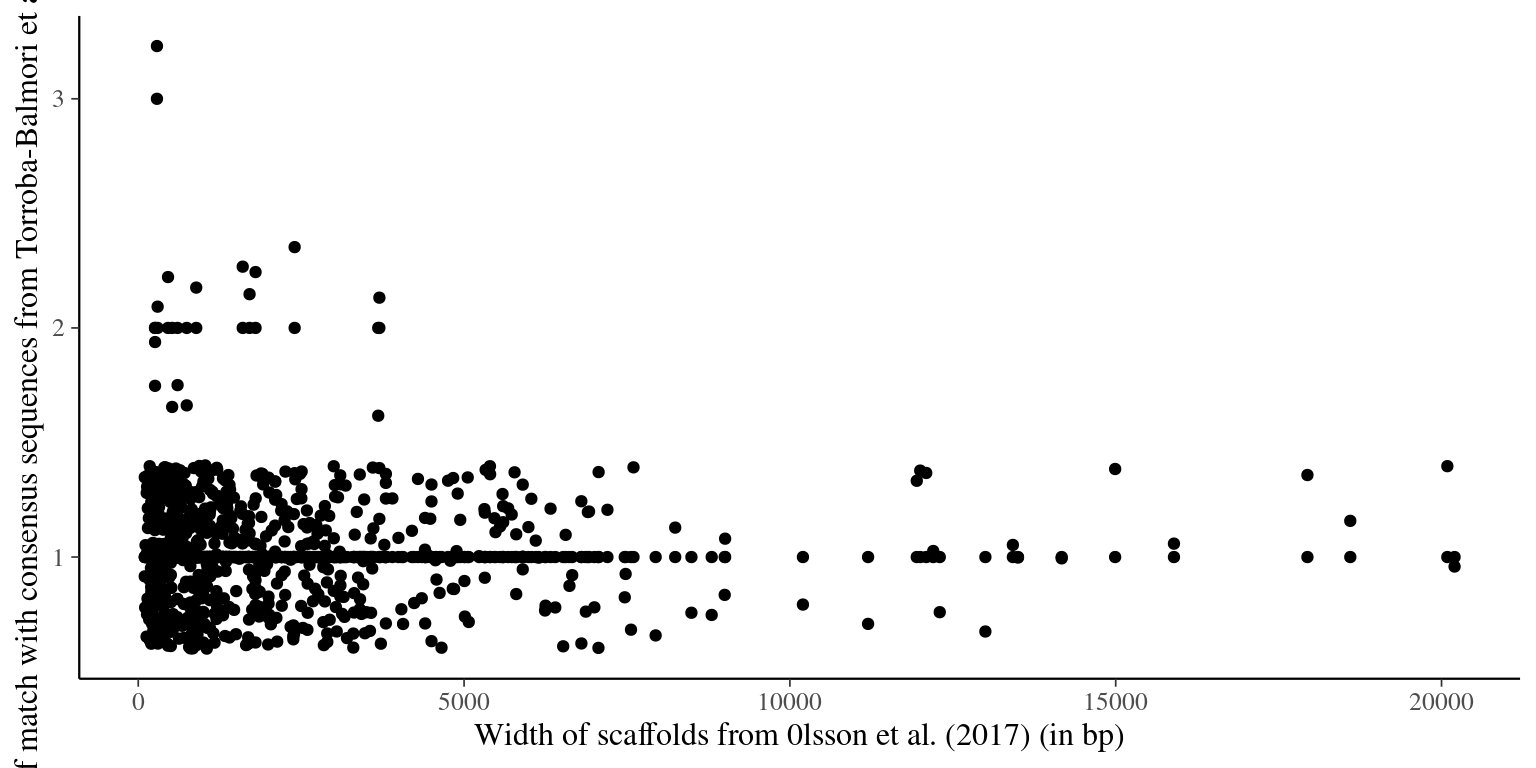
Figure 2.2: Number of matches with Torroba-Balmori’s consensus reads vs gene width.
| Scaffold | width | remove | cut |
|---|---|---|---|
| Olsson_2017_deg7180004393135 | 2380 | 1700-1631 | |
| Olsson_2017_deg7180004374686 | 2120 | 2073-1992 | |
| Olsson_2017_scf7180005372912 | 3152 | 3102-3152 | |
| Olsson_2017_scf7180005387046 | 2048 | 174-256 | |
| Olsson_2017_scf7180005323991 | 2482 | 2330-2267 |
The following scaffolds have been removed due to multiple matches and a length \(<200bp\): deg7180004378417, deg7180003744575, deg7180002657883, deg7180004705895, deg7180004369764, deg7180002776754, deg7180004453462, deg7180004453461, deg7180002668453, deg7180005298947, deg7180003723902, deg7180005298948, deg7180004372504, deg7180002659849, deg7180004372505, deg7180004377385, deg7180003260802, deg7180003625436, deg7180004705895, deg7180002776754, deg7180004705894, deg7180002852093, deg7180004822905, deg7180005023024, deg7180004478675, deg7180004428004, deg7180004428003, deg7180004507379, deg7180002656221, deg7180004374687, deg7180004372498, deg7180004372497, deg7180002654368, deg7180002674357, deg7180004700334, deg7180004899808, deg7180004899808, deg7180002726303, scf7180005372913, deg7180005163225, deg7180003214542, scf7180005400822, deg7180005163224, deg7180003138164, deg7180004981997, deg7180004981996, deg7180005171251, deg7180005106503, deg7180003910181, deg7180005026532, deg7180003853280, deg7180004724986, deg7180005246885, deg7180004710959, deg7180004681149, deg7180004580422, deg7180004472718, deg7180003290510, deg7180005004768, deg7180004756559, scf7180005435685, deg7180004725719, deg7180004599019, deg7180004599018, deg7180002749392, deg7180002739372, deg7180004754314, deg7180004847375, deg7180004580009, deg7180004386399, deg7180004377195, deg7180004377194, deg7180004399409, deg7180004392029, deg7180004385805, deg7180004386398, deg7180002816623, deg7180002985310, scf7180005421751, deg7180004374725, deg7180004372798, deg7180004374726, deg7180002668107, deg7180003199928, deg7180003093903, deg7180003310549, deg7180004796671, deg7180003505925, deg7180002988969. And other have been cut (see table 2.2).
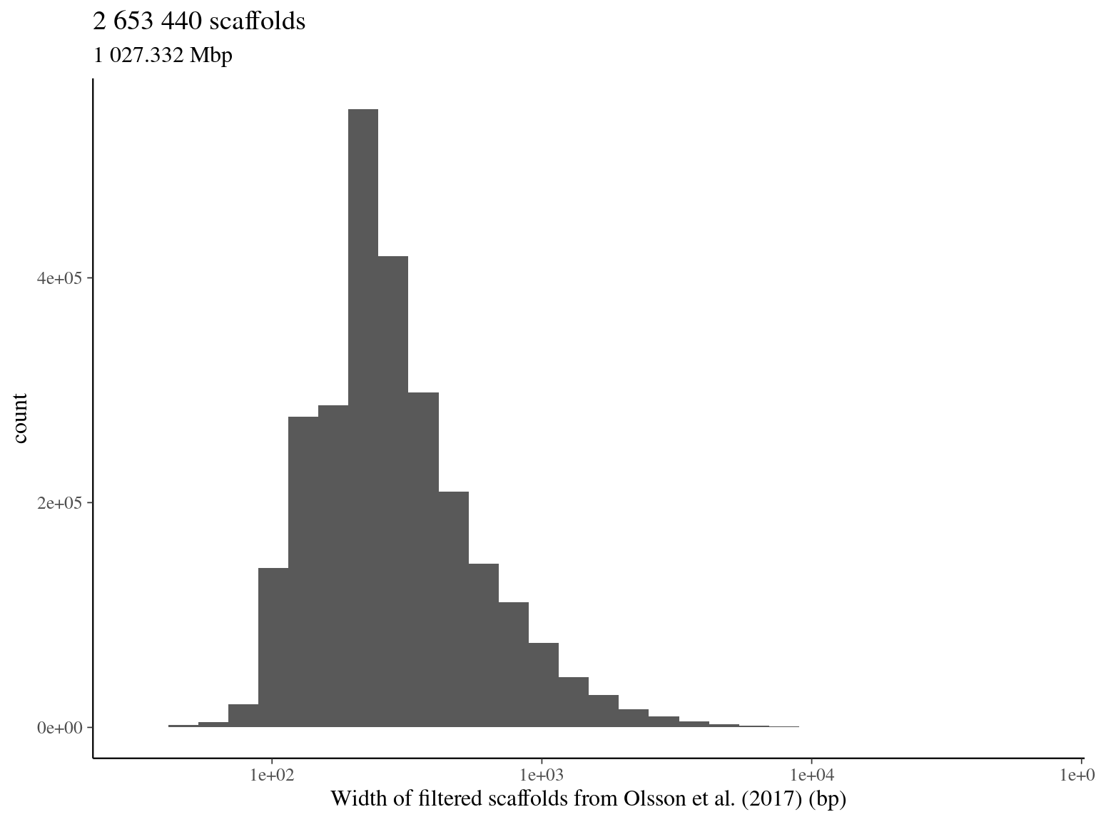
2.2.3 Total filtered scaffolds
2.3 Tysklind et al (in prep) transcript preparation
Tysklind et al (in prep) used 20 Symphonia juveniles from the transplantation garden experiment for transcriptomic analysis.
RNA sequences were captured.
The analysis followed the scheme suggested by Lopez-Maestre et al. (2016) (see below).
First, reads were assembled with Trinity into transcripts.
In parallel, SNPs were detected with Kissplice.
Then SNPs were mapped on the transcriptome with BLAT.
In parallel SNPs have been tested to be morphotype-specific at the level \(\alpha = 0.001\) with KissDE and transcriptome Open Reading Frames (ORF) have been identified with Transdecoder.
Finally, SNPs with a functional impact were identified through k2rt.
Consequently, for every SNP we have the following information:
(i) inside coding DNA sequence (CDS),
(ii) synonymous or not,
(iii) morphotype-specificity.
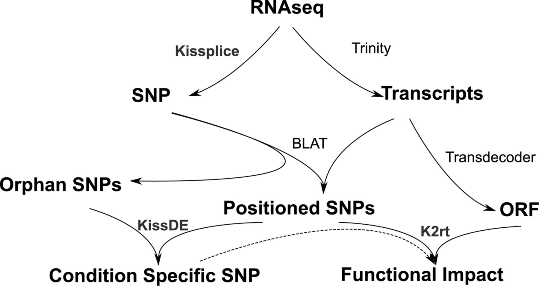
Analysis scheme from Lopez-Maestre et al. (2016).
2.3.1 Filtering SNP on quality
We assessed transcriptomic analysis quality with possible sequencing errors, and SNPs in multiple assembled genes or isoforms (see table 2.3). We found 38 594 SNPs with possible sequencing error, and 609 214 SNPs associated to multiple assembled genes that we removed from further analysis.
| variable | n | Percentage |
|---|
2.3.2 Filtering SNP on type
We also highlighted SNPs which met impossible association of characteristic (table 2.4), that we removed from further analysis.
| Coding sequence | Not synonymous | Morphotype-specific | n | type |
|---|
2.3.3 Filtering transcripts on SNP frequency
We found a high frequency of SNPs per candidate gene (the majority between 1 SNP per 10 or 100 bp), with some scaffolds having a SNP frequency superior to 0.2 (see figure 2.3). We assumed those hyper SNP-rich scaffolds to be errors and decided to remove them from the reference transcriptome. In order to do that, we fitted a \(\Gamma\) law into the SNP frequency distribution and we kept scaffolds with a SNP frequency under the \(99^{th}\) quantile (\(q_{99} = 0.07810194\)). We thus removed:
- 358 308 SNPs
- located on 20 521 transcripts
- representing 1 490 candidate genes
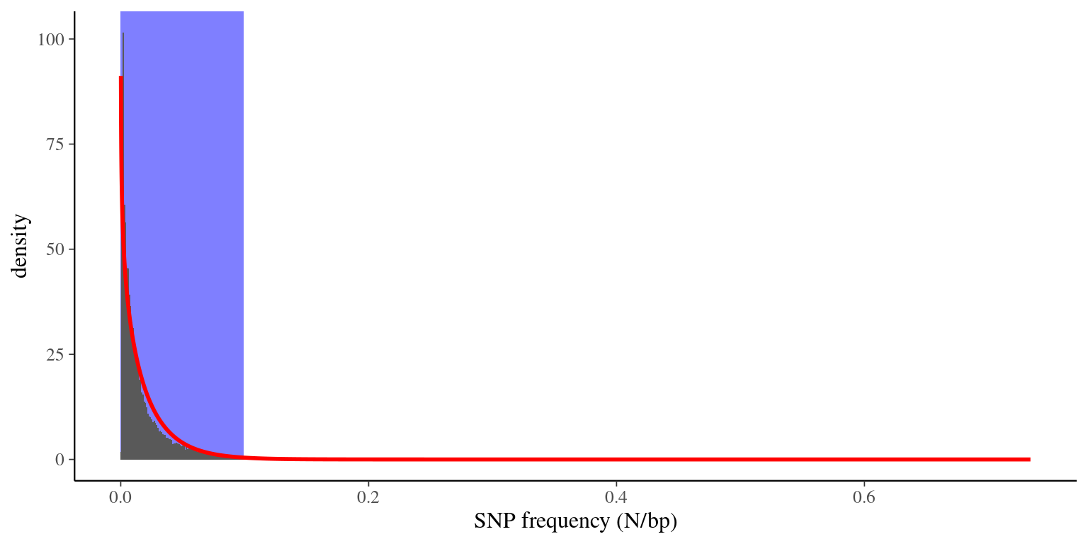
Figure 2.3: Distribution of SNP frequencies in scaffolds. Histogram (grey bars) represents the data, red line represents the Gamma law fit, and blue area represents X*sigma where scaffolds are not excluded.
filtered_data <- snp_genes %>%
  filter(freq <= q99) %>%
  left_join(data, by = "gene_id") %>%
  select(transcript_id, sequence) %>%
  unique() %>%
  mutate(transcript_id = paste0(">", transcript_id))
filtered_data_fasta <- do.call(rbind, lapply(seq(nrow(filtered_data)),
                                             function(i) t(filtered_data[i, ])))
write.table(filtered_data_fasta, row.names = F, col.names = F, quote = F,
            file = file.path(path, "..", "filtered_transcripts.fasta"))
2.3.4 Total filtered transcript
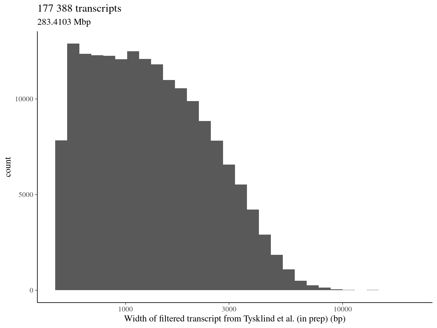
We have a total of:
- 1 382 525 filtered SNPs (over 2 398 550)
- located on 177 388 transcripts (over 257 140, when pseudo-genes and isoforms)
- representing 63 707 candidate genes (over 76 032, respectively)
- for a total of 283.4 Mbp
2.4 Neutral region selection
2.4.1 Raw reads from Torroba-Balmori et al. (unpublished) alignment on scaffolds from Scotti et al. (in prep)
We used the French Guianan raw reads from Torroba-Balmori et al. (unpublished),
by aligning them on scaffolds from Olsson et al. (2017) with bwa.
#!/bin/bash
#SBATCH --time=36:00:00
#SBATCH -J alignIvan
#SBATCH -o alignIvan_output.out
#SBATCH -e alignIvan_error.out
#SBATCH --mem=20G
#SBATCH --cpus-per-task=1
#SBATCH --mail-type=BEGIN,END,FAIL

# Environment
module purge
module load bioinfo/bwa-0.7.15
module load bioinfo/picard-2.14.1
module load bioinfo/samtools-1.4
module load bioinfo/bedtools-2.26.0

# read preparation
cd ~/work/Symphonia_Torroba/
tar -xvzf Gbs.tar.gz
cd raw
rm PR_49.fastq RG_1.fastq
for file in ./*.fastq
do
  echo $file
  filename=$(basename "$file")
  filename="${filename%.*}"
  perl -pe 's|[\h]||g' $file > "${filename}".renamed.fastq
  rm $file
done
# variables
cd ~/work/Symphonia_Genomes/Ivan_2018/torroba_alignment
reference=~/work/Symphonia_Genomes/Ivan_2018/merged_1000/merged_1000.fa
query_path=~/work/Symphonia_Torroba/raw
# alignment
bwa index $reference
mkdir bwa
for file in $query_path/*.fastq
do
  filename=$(basename "$file")
  filename="${filename%.*}"
  rg="@RG\tID:${filename}\tSM:${filename}\tPL:IONTORRENT"
  bwa mem -M -R "${rg}" $reference $file > bwa/"${filename}.sam"
#  rm $file
done
# sam2bam
for file in ./bwa/*.sam
do
  filename=$(basename "$file")
  filename="${filename%.*}"
  java -Xmx4g -jar $PICARD SortSam I=$file O=bwa/"${filename}".bam SORT_ORDER=coordinate
done
# Bam index
for file in bwa/*.bam
do
  filename=$(basename "$file")
  filename="${filename%.*}"
  java -Xmx4g -jar $PICARD BuildBamIndex I=$file O=bwa/"${filename}".bai
done
# sam2bed
mkdir bed
for file in ./bwa/*.bam
do
  filename=$(basename "$file")
  filename="${filename%.*}"
  bedtools bamtobed -i bwa/"${filename}".bam > bed/"${filename}".bed
done
# merge bed
mkdir merged_bed
for file in ./bed/*.bed
do
  filename=$(basename "$file")
  filename="${filename%.*}"
  bedtools merge -i bed/"${filename}".bed > merged_bed/"${filename}".bed
done
cat bed/* | sort -k 1,1 -k2,2n >  all.nonunique.bed
bedtools merge -i all.nonunique.bed -c 1 -o count > all.merged.bed
bed <- read_tsv(file.path(path, "Ivan_2018", "torroba_alignment", "all.merged.bed"), col_names = F)
names(bed) <- c("scaffold", "start", "end", "coverage")
write_file(paste(unique(bed$scaffold), collapse = "\n"),
file.path(path, "Ivan_2018", "torroba_alignment", "scaffolds.list"))cd ~/Documents/BIOGECO/PhD/data/Symphonia_Genomes/Ivan_2018/torroba_alignment
ref=~/Documents/BIOGECO/PhD/data/Symphonia_Genomes/Ivan_2018/merged_1000/merged_1000.fa
seqtk subseq $ref scaffolds.list >> scaffolds.fa| N | Width (Mbp) | Coverage (%) | |
|---|---|---|---|
| aligned sequence | 1 786 852 | 130.3105 | 29.87923 |
| selected scaffold | 179 665 | 421.7514 | 96.70448 |
| total | 190 098 | 436.1239 | 100.00000 |
2.4.2 Masking scaffolds with multimatch from Scotti et al. (in prep)
bed <- data.table::fread(file.path(path, "Ivan_2018", "torroba_alignment",
                                   "all.nonunique.bed"), header = F)
names(bed) <- c("scaffold", "start", "end", "read", "quality", "orientation")
multimatch_reads <- bed %>%
  filter(duplicated(read)) %>%
  select(read) %>%
  unique() %>%
  unlist()
bed %>%
  filter(read %in% multimatch_reads) %>%
  write_tsv(file.path(path, "Ivan_2018", "torroba_alignment",
                       "multimatch.bed"), col_names = F)
rm(bed, multimatch_reads) ; invisible(gc())
cd ~/Documents/BIOGECO/PhD/data/Symphonia_Genomes/Ivan_2018/torroba_alignment
bedtools maskfasta -fi scaffolds.fa -bed multimatch.bed -fo masked.scaffolds.fascf <- readDNAStringSet(file.path(path, "Ivan_2018",
"torroba_alignment", "masked.scaffolds.fa"))
scf <- data.frame(scaffold = names(scf), width = width(scf),
N = letterFrequency(scf, letters = "N")) %>%
mutate(Nperc = N/width*100) %>%
filter(Nperc < 25 & width > 1000) %>%
select(scaffold)
write_file(paste(scf$scaffold, collapse = "\n"),
file.path(path, "Ivan_2018", "torroba_alignment", "final.scaffolds.list"))cd ~/Documents/BIOGECO/PhD/data/Symphonia_Genomes/Ivan_2018/torroba_alignment
seqtk subseq masked.scaffolds.fa final.scaffolds.list >> final.scaffolds.fa| N | Width (Mbp) | Mask (%N) | Coverage (%) | |
|---|---|---|---|---|
| selected scaffold | 315 226 | 776.5915 | 6.651114 | 178.0667 |
| total | 190 098 | 436.1239 | NA | 100.0000 |
2.4.3 Raw reads from Torroba-Balmori et al. (unpublished) alignment on scaffolds from Olsson et al. (2017)
We used again the French Guianan raw reads from Torroba-Balmori et al. (unpublished),
to align them on scaffolds from Olsson et al. (2017) with bwa.
#!/bin/bash
#SBATCH --time=36:00:00
#SBATCH -J alignOlsson
#SBATCH -o alignOlsson_output.out
#SBATCH -e alignOlsson_error.out
#SBATCH --mem=20G
#SBATCH --cpus-per-task=1
#SBATCH --mail-type=BEGIN,END,FAIL

# Environment
module purge
module load bioinfo/bwa-0.7.15
module load bioinfo/picard-2.14.1
module load bioinfo/samtools-1.4
module load bioinfo/bedtools-2.26.0

# read preparation
cd ~/work/Symphonia_Torroba/
tar -xvzf Gbs.tar.gz
cd raw
rm PR_49.fastq RG_1.fastq
for file in ./*.fastq
do
  echo $file
  filename=$(basename "$file")
  filename="${filename%.*}"
  perl -pe 's|[\h]||g' $file > "${filename}".renamed.fastq
  rm $file
done
# variables
cd ~/work/Symphonia_Genomes/Olsson_2016/torroba_alignment
reference=~/work/Symphonia_Genomes/Olsson_2016/Olsson2017/Olsson2017.fa
query_path=~/work/Symphonia_Torroba/raw
# alignment
bwa index $reference
mkdir bwa
for file in $query_path/*.fastq
do
  filename=$(basename "$file")
  filename="${filename%.*}"
  rg="@RG\tID:${filename}\tSM:${filename}\tPL:IONTORRENT"
  bwa mem -M -R "${rg}" $reference $file > bwa/"${filename}.sam"
  rm $file
done
# sam2bam
for file in ./bwa/*.sam
do
  filename=$(basename "$file")
  filename="${filename%.*}"
  java -Xmx4g -jar $PICARD SortSam I=$file O=bwa/"${filename}".bam SORT_ORDER=coordinate
done
# Bam index
for file in bwa/*.bam
do
  filename=$(basename "$file")
  filename="${filename%.*}"
  java -Xmx4g -jar $PICARD BuildBamIndex I=$file O=bwa/"${filename}".bai
done
# sam2bed
mkdir bed
for file in ./bwa/*.bam
do
  filename=$(basename "$file")
  filename="${filename%.*}"
  bedtools bamtobed -i bwa/"${filename}".bam > bed/"${filename}".bed
done
# merge bed
mkdir merged_bed
for file in ./bed/*.bed
do
  filename=$(basename "$file")
  filename="${filename%.*}"
  bedtools merge -i bed/"${filename}".bed > merged_bed/"${filename}".bed
done
cat bed/* | sort -k 1,1 -k2,2n >  all.nonunique.bed
bedtools merge -i all.nonunique.bed -c 1 -o count > all.merged.bed
bed <- read_tsv(file.path(path, "Olsson_2016", "torroba_alignment", "all.merged.bed"), col_names = F)
names(bed) <- c("scaffold", "start", "end", "coverage")
write_file(paste(unique(bed$scaffold), collapse = "\n"),
file.path(path, "Olsson_2016", "torroba_alignment", "scaffolds.list"))cd ~/Documents/BIOGECO/PhD/data/Symphonia_Genomes/Olsson_2016/torroba_alignment
ref=~/Documents/BIOGECO/PhD/data/Symphonia_Genomes/Olsson_2016/Olsson2017/Olsson2017.fa
seqtk subseq $ref scaffolds.list >> scaffolds.fa| N | Width (Mbp) | Coverage (%) | |
|---|---|---|---|
| aligned sequence | 1 786 852 | 130.3105 | 12.68385 |
| selected scaffold | 1 056 548 | 590.1957 | 57.44708 |
| total | 2 653 526 | 1 027.3729 | 100.00000 |
2.4.4 Masking scaffolds with multimatch from Olsson et al. (2017)
bed <- data.table::fread(file.path(path, "Olsson_2016", "torroba_alignment",
                                   "all.nonunique.bed"), header = F)
names(bed) <- c("scaffold", "start", "end", "read", "quality", "orientation")
multimatch_reads <- bed %>%
  filter(duplicated(read)) %>%
  select(read) %>%
  unique() %>%
  unlist()
bed %>%
  filter(read %in% multimatch_reads) %>%
  write_tsv(file.path(path, "Olsson_2016", "torroba_alignment",
                       "multimatch.bed"), col_names = F)
rm(bed, multimatch_reads) ; invisible(gc())
cd ~/Documents/BIOGECO/PhD/data/Symphonia_Genomes/Olsson_2016/torroba_alignment
bedtools maskfasta -fi scaffolds.fa -bed multimatch.bed -fo masked.scaffolds.fascf <- readDNAStringSet(file.path(path, "Olsson_2016",
"torroba_alignment", "masked.scaffolds.fa"))
scf <- data.frame(scaffold = names(scf), width = width(scf),
N = letterFrequency(scf, letters = "N")) %>%
mutate(Nperc = N/width*100) %>%
filter(Nperc < 25 & width > 1000) %>%
select(scaffold)
write_file(paste(scf$scaffold, collapse = "\n"),
file.path(path, "Olsson_2016", "torroba_alignment", "final.scaffolds.list"))cd ~/Documents/BIOGECO/PhD/data/Symphonia_Genomes/Olsson_2016/torroba_alignment
ref=~/Documents/BIOGECO/PhD/data/Symphonia_Genomes/Olsson_2016/Olsson2017/Olsson2017.fa
seqtk subseq masked.scaffolds.fa final.scaffolds.list >> final.scaffolds.fa| N | Width (Mbp) | Mask (%N) | Coverage (%) | |
|---|---|---|---|---|
| selected scaffold | 245 646 | 464.1304 | 1.896894 | 45.17643 |
| total | 2 653 526 | 1 027.3729 | NA | 100.00000 |
2.4.5 Removing scaffolds already matching transcripts
func <-unlist(read_tsv(file.path(path, "Ivan_2018",
                          "transcript_alignment", "selected_scaffolds.list"), col_names = F))
neutral <- readDNAStringSet(file.path(path, "Ivan_2018", "torroba_alignment",
                                  "final.scaffolds.fa"))
writeXStringSet(neutral[setdiff(names(neutral), func)], file.path(path, "neutral_selection", "Ivan.selected.scaffolds.fa"))
func <-unlist(read_tsv(file.path(path, "Olsson_2016",
"transcript_alignment", "selected_scaffolds.list"), col_names = F))
neutral <- readDNAStringSet(file.path(path, "Olsson_2016", "torroba_alignment",
"final.scaffolds.fa"))
writeXStringSet(neutral[setdiff(names(neutral), func)], file.path(path, "neutral_selection", "Olsson.selected.scaffolds.fa"))2.4.6 Merge of selected scaffolds
We merged selected scaffolds from Scotti et al (in prep) and Olsson et al. (2017) with quickmerge.
cd ~/Documents/BIOGECO/PhD/data/Symphonia_Genomes/neutral_selection
ref=Ivan.selected.scaffolds.fa
query=Olsson.selected.scaffolds.fa
nucmer -l 100 -prefix out $ref $query
delta-filter -i 95 -r -q out.delta > out.rq.delta
~/Tools/quickmerge/quickmerge -d out.rq.delta -q $query -r $ref -hco 5.0 -c 1.5 -l n -ml m
We merged selected scaffolds from Scotti et al (in prep) and Olsson et al. (2017) with quickmerge.
We found 13 343 overlaps resulting a final merged assembly of 82 792 scaffolds for a total length of 146.80 Mb.
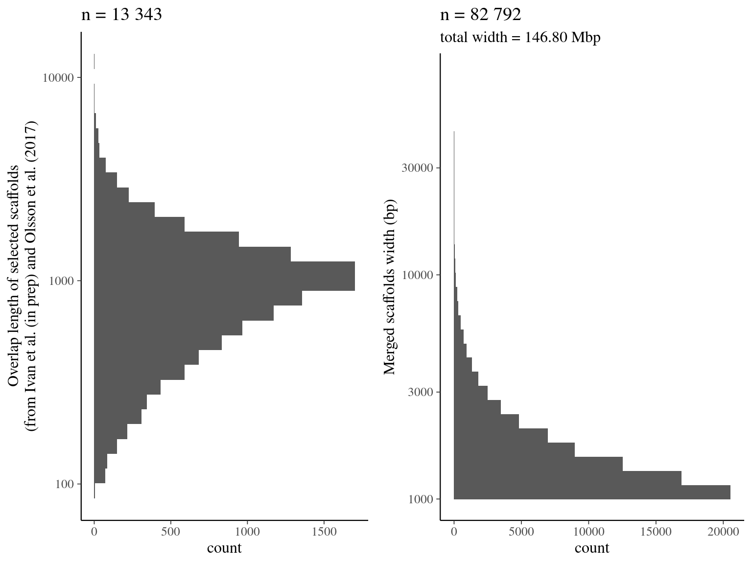
Figure 2.4: Merging result from quickmerge. Left graph represents the overlap distribution. Right graph represent the merged scaffolds distribution.
2.4.7 Final subset of selected neutral scaffolds
We finally selected 0.533 Mb of sequences by sampling 533 1-kb sequences among 533 scaffolds (1 sequence per scaffold) with a probability \(p=\frac{scaffold\_length}{total\_length}\).
scf <- readDNAStringSet(file.path(path, "neutral_selection", "merged.fasta"))
selection <- data.frame(scf = names(scf), width = width(scf),
                        N = letterFrequency(scf, "N")) %>%
  sample_n(533, weight = width) %>%
  select(scf) %>%
  unlist()
scf_sel <- subseq(scf[selection], end=1000, width=1000)
writeXStringSet(scf_sel, file.path(path, "neutral_selection", "selected.scaffolds.fa"))| N | Width (Mbp) | Mask (%N) |
|---|---|---|
| 533 | 0.533 | 0.0036529 |
2.4.8 Repetitive regions final check
Last but not least, we do not want to include repetitive regions in our targets for baits design. We consequently aligned raw reads from one library from Scotti et al. (in prep) on our targets with bwa.
cd ~/Documents/BIOGECO/PhD/data/Symphonia_Genomes/neutral_selection
reference=selected.scaffolds.fa
query=~/Documents/BIOGECO/PhD/data/Symphonia_Genomes/Ivan_2018/raw_reads/globu1_symphonia_globulifera_CTTGTA_L001_R1_001.fastq.gz
bwa index $reference
bwa mem -M $reference $query > raw_read_alignment.sam
picard=~/Tools/picard/picard.jar
java -Xmx4g -jar $picard SortSam I=raw_read_alignment.sam O=raw_read_alignment.bam SORT_ORDER=coordinate
bedtools bamtobed -i raw_read_alignment.bam > raw_read_alignment.bed
cat raw_read_alignment.bed | sort -k 1,1 -k2,2n >  raw_read_alignment.sorted.bed
bedtools merge -i raw_read_alignment.sorted.bed -c 1 -o count > raw_read_alignment.merged.bed
We obtained a continuous decreasing distribution of read coverage across our scaffolds regions (figure 2.5). We fitted a \(\Gamma\) distribution with positive parameters for scaffolds regions with a coverage under 5 000 (non continuous distribution with optimization issues). We obtained a distribution with a mean of 324 reads per region and a \(99^{th}\) quantile of 4 042. We decided to mask regions with a coverage over the \(99^{th}\) quantile and remove scaffolds with a mask superior to 75% of its total length (figure 2.5).
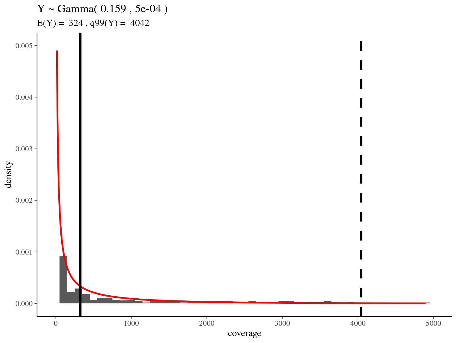
Figure 2.5: Read coverage distribution.
repetitive_target <- bed %>%
  filter(coverage > qgamma(0.99, alpha, beta)) %>%
  mutate(size = end - start)
repetitive_target %>%
  select(target, start, end) %>%
  arrange(target, start, end) %>%
  mutate_if(is.numeric, as.character) %>%
  write_tsv(path = file.path(path, "neutral_selection", "repetitive_targets.bed"),
            col_names = F)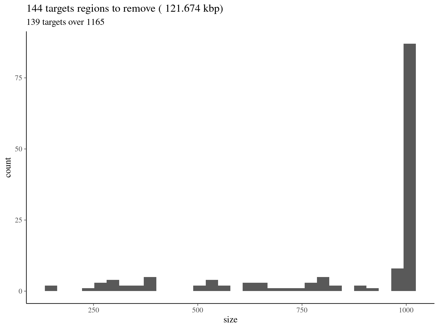
Figure 2.6: target regions with a coverage over the 99th quantile of the fitted Gamma distribution (4042).
cd ~/Documents/BIOGECO/PhD/data/Symphonia_Genomes/neutral_selection
cat repetitive_targets.bed | sort -k 1,1 -k2,2n >  repetitive_targets.sorted.bed
bedtools maskfasta -fi selected.scaffolds.fa -bed repetitive_targets.sorted.bed -fo targets.masked.fasta
targets <- readDNAStringSet(file.path(path, "neutral_selection", "targets.masked.fasta"))
writeXStringSet(targets[which(letterFrequency(targets, "N")/width(targets) < 0.65)],
file.path(path, "neutral_selection", "targets.filtered.masked.fasta"))| N | Width (Mbp) | Mask (%N) |
|---|---|---|
| 415 | 0.415 | 0.024412 |
2.5 Fuctional region selection
We used open reading frames (ORF) to target genes within scaffolds.
ORFs have been detected with transdecoder on assembled transcripts.
First, we filtered ORFs including a start codon(figure 2.7).
Then, we aligned ORFs on pre-selected and merged genomic scaffolds with blat.
We obtained 7 744 aligned scaffolds (table 2.11 and figure 2.8).
Thanks to alignments, we removed overlapping genes (figure 2.9) and obtained 4 076 pre-selected genes with a total length of 757 kbp (figure 2.10).
Finally, we used transcript differential expression to select all genes differentially expressed between Symphonia globulifera and Symphonia sp1 (figure 2.11).
We selected 1150 sequences of 500 to 1-kbp representing 1 063 Mbp (table 2.12).
To validate our final target set, we aligned with bwa raw reads from one library from Scotti et al. (in prep).
2.5.1 Open Reading Frames (ORFs) filtering
173 828 ORFs including a start codon (Methyonin, M) were detected (over 231 883, 75%, see figure 2.7.
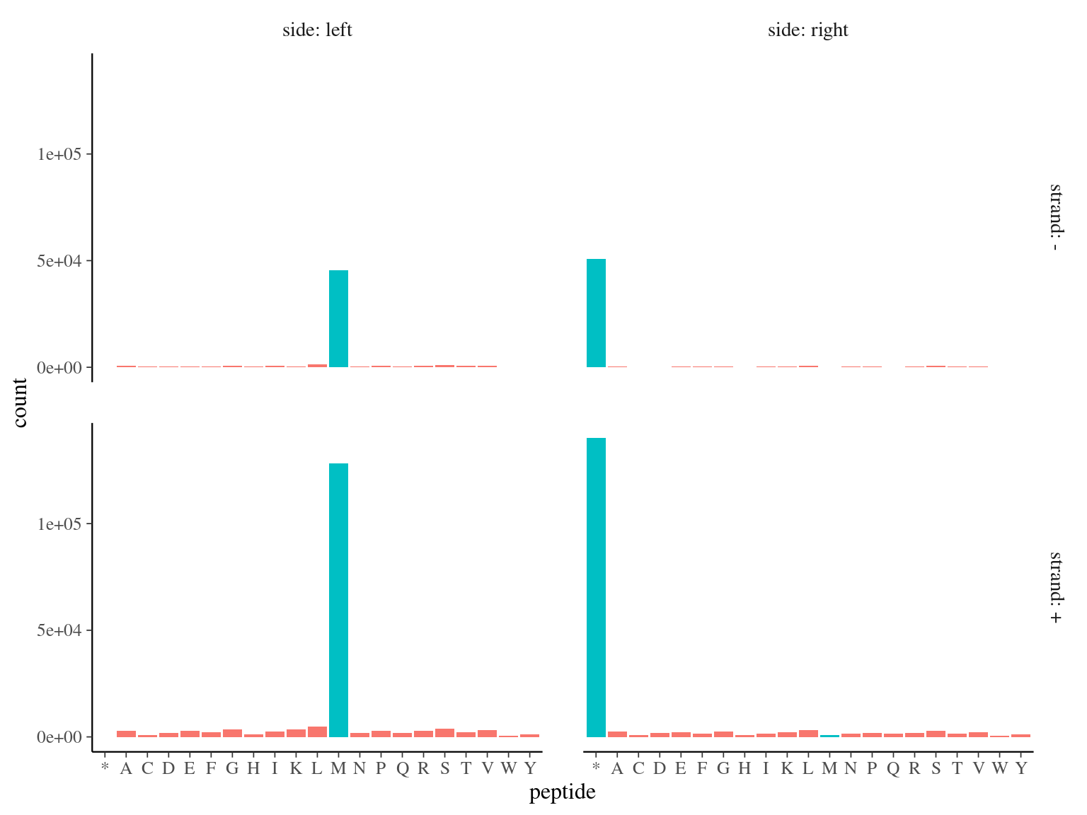
Figure 2.7: Open Reading Frames left and right peptides.
orf <- src_sqlite(file.path(path, "Niklas_transcripts/Trinotate/",
                           "symphonia.trinity500.trinotate.sqlite")) %>%
  tbl("ORF") %>%
  dplyr::rename(orf = orf_id, trsc = transcript_id,
                orfSize = length) %>%
  filter(substr(peptide, 1, 1) == "M") %>%
  select(-peptide, -strand) %>%
  collect() %>%
  rowwise() %>%
  mutate(orfStart = min(as.numeric(lend), as.numeric(rend)),
         orfEnd = max(as.numeric(lend), as.numeric(rend))) %>%
  select(-lend, -rend) %>%
  select(trsc, orfStart, orfEnd, orf) %>%
  mutate_if(is.numeric, as.character) %>%
  write_tsv(path = file.path(path, "functional_selection2", "orf.all.bed"),
            col_names = F)
2.5.2 ORF alignment on genomics scaffolds
7 744 scaffolds matched with ORFs (10.5% for 15.4 Mbp, see table 2.11 and figure 2.8).
cd ~/Documents/BIOGECO/PhD/data/Symphonia_Genomes/functional_selection2
cat orf.all.bed | sort -k 1,1 -k2,2n >  orf.all.sorted.bed
trsc=/home/sylvain/Documents/BIOGECO/PhD/data/Symphonia_Niklas/filtered_transcripts.fasta
bedtools getfasta -name -fi $trsc -bed orf.all.sorted.bed -fo orf.fasta
scf=~/Documents/BIOGECO/PhD/data/Symphonia_Genomes/neutral_selection/merged.fasta
orf=./orf.fasta
blat $scf $orf alignment.psl| N | Width (Mbp) | Coverage (%) | |
|---|---|---|---|
| aligned sequence | 21 146 | 2.201315 | 1.499565 |
| selected scaffold | 7 744 | 15.425248 | 10.507881 |
| total | 82 792 | 146.796946 | 100.000000 |
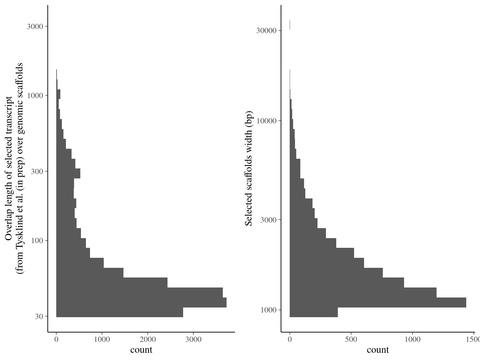
Figure 2.8: Alignment result of Tysklind et al. (in prep) ORFs over genomic scaffolds with blat. Left graph represents the overlap distribution. Right graph represent the selected and deduplicated scaffolds distribution.
2.5.3 Overlaping genes filtering
995 genes were overlapping and filtered out (figure 2.9).
alignment %>%
  separate(orf, into = c("gene", "isoform", "geneNumber", "orfNumber"),
           sep = "::", remove = F) %>%
  select(gene, orf, orfStart, orfEnd, scf, scfStart, scfEnd) %>%
  unique() %>%
  select(scf, scfStart, scfEnd, orf, gene) %>%
  arrange(scf, scfStart, scfEnd) %>%
  mutate_if(is.numeric, as.character) %>%
  write_tsv(path = file.path(path, "functional_selection2", "genes.all.bed"),
            col_names = F)
cd ~/Documents/BIOGECO/PhD/data/Symphonia_Genomes/functional_selection2
cat genes.all.bed | sort -k 1,1 -k2,2n > genes.all.sorted.bed
bedtools merge -i genes.all.sorted.bed -c 5 -o collapse > genes.merged.bed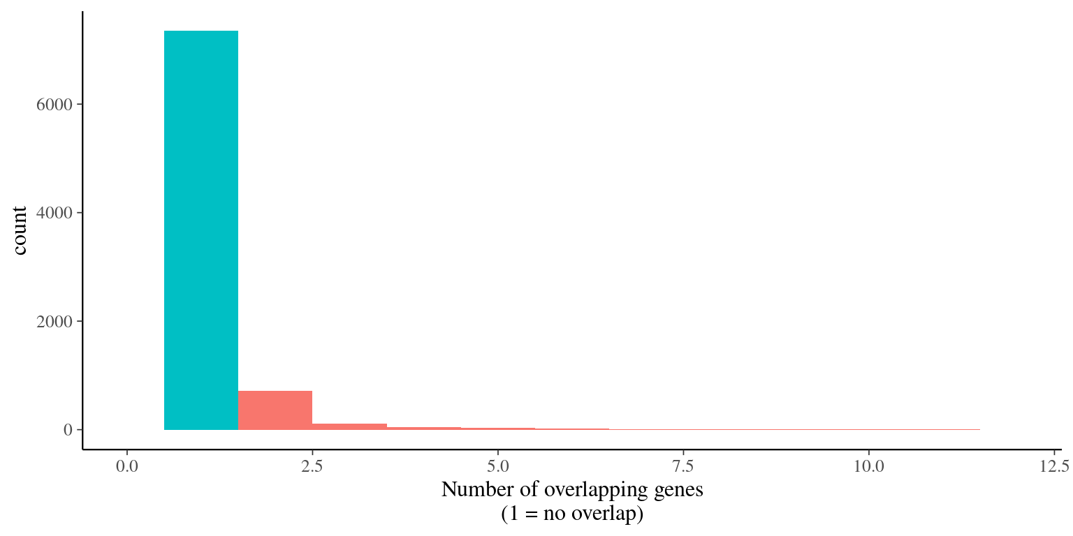
Figure 2.9: Genes overlap
2.5.4 Pre-selected genes
We obtained 4 076 genes pre-selected for a total length of 757 kbp (figure 2.10).
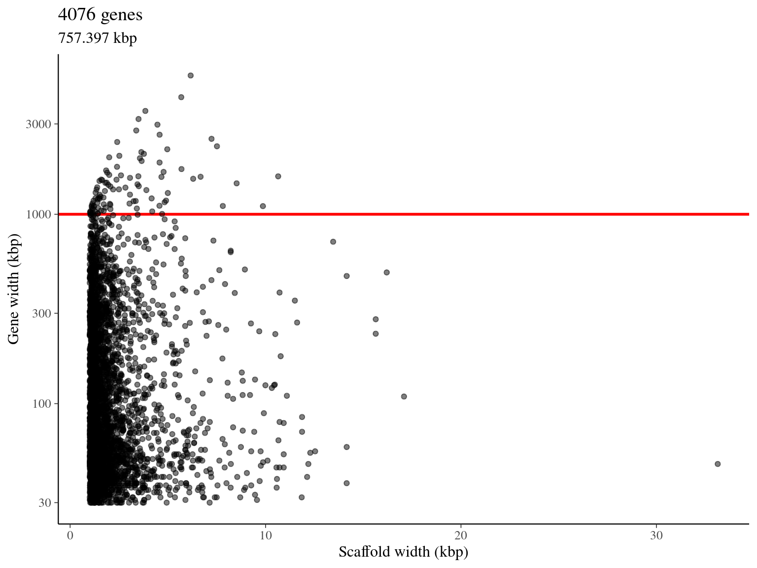
Figure 2.10: Available genes for target sequences design.
2.5.5 Differential Expression (DE) of genes
Figure 2.11 shows genes differential expression. First circle represents genes with isoforms not enriched whereas second and third circle represent, respectively, genes with isoforms S. sp1 and S. globulifera enriched. Relatively few genes contained enriched isoforms, and most of them were S. globulifera enriched.
Figure 2.11: Genes differential expression.
2.5.6 Final subset of selected functional scaffolds
We finally selected 1150 sequences of 500 to 1-kbp with 100 bp before geneStart and a maximum of 900 bp after, resulting in 1 063, 544 kbp of targets. All differentially expressed genes between morphotypes were selected (159). And the rest of sequences were randomly selected among non differentially expressed genes (1001).
targets <- genes %>%
  left_join(de) %>%
  filter(deg %in% c("Eglo", "Esp")) %>%
  rbind(genes %>%
          left_join(de) %>%
          filter(deg %in% c("DE", NA)) %>%
          sample_n(1309)) %>%
  group_by(scf, gene) %>%
  filter(n() < 2) %>%
  mutate(targetStart = max(0, geneStart - 100)) %>%
  mutate(targetEnd = min(targetStart + 1000, scfSize)) %>%
  mutate(targetSize = targetEnd - targetStart) %>%
  filter(targetSize > 500) %>%
  mutate(target = paste0(gene, "_on_", scf)) %>%
  ungroup()
targets %>%
  select(scf, targetStart, targetEnd, target) %>%
  arrange(scf, targetStart, targetEnd, target) %>%
  mutate_if(is.numeric, as.character) %>%
  write_tsv(path = file.path(path, "functional_selection2", "targets.all.bed"),
            col_names = F)
cd ~/Documents/BIOGECO/PhD/data/Symphonia_Genomes/functional_selection2
cat targets.all.bed | sort -k 1,1 -k2,2n > targets.all.sorted.bed
scf=~/Documents/BIOGECO/PhD/data/Symphonia_Genomes/neutral_selection/merged.fasta
bedtools getfasta -name -fi $scf -bed targets.all.sorted.bed -fo targets.fasta| N | Width (Mbp) | Mask (%N) |
|---|---|---|
| 1 165 | 1.068207 | 0.0025285 |
2.5.7 Repetitive regions final check
Last but not least, we do not want to include repetitive regions in our targets for baits design. We consequently aligned raw reads from one library from Scotti et al. (in prep) on our targets with bwa.
cd ~/Documents/BIOGECO/PhD/data/Symphonia_Genomes/functional_selection2
reference=targets.fasta
query=~/Documents/BIOGECO/PhD/data/Symphonia_Genomes/Ivan_2018/raw_reads/globu1_symphonia_globulifera_CTTGTA_L001_R1_001.fastq.gz
bwa index $reference
bwa mem -M $reference $query > raw_read_alignment.sam
picard=~/Tools/picard/picard.jar
java -Xmx4g -jar $picard SortSam I=raw_read_alignment.sam O=raw_read_alignment.bam SORT_ORDER=coordinate
bedtools bamtobed -i raw_read_alignment.bam > raw_read_alignment.bed
cat raw_read_alignment.bed | sort -k 1,1 -k2,2n >  raw_read_alignment.sorted.bed
bedtools merge -i raw_read_alignment.sorted.bed -c 1 -o count > raw_read_alignment.merged.bed
We obtained a continuous decreasing distribution of read coverage across our scaffolds regions (figure 2.12). We fitted a \(\Gamma\) distribution with positive parameters for scaffolds regions with a coverage under 5 000 (non continuous distribution with optimization issues). We obtained a distribution with a mean of 309 reads per region and a \(99^{th}\) quantile of 2 606. We decided to mask regions with a coverage over the \(99^{th}\) quantile and remove scaffolds with a mask superior to 75% of its total length (figure 2.12).
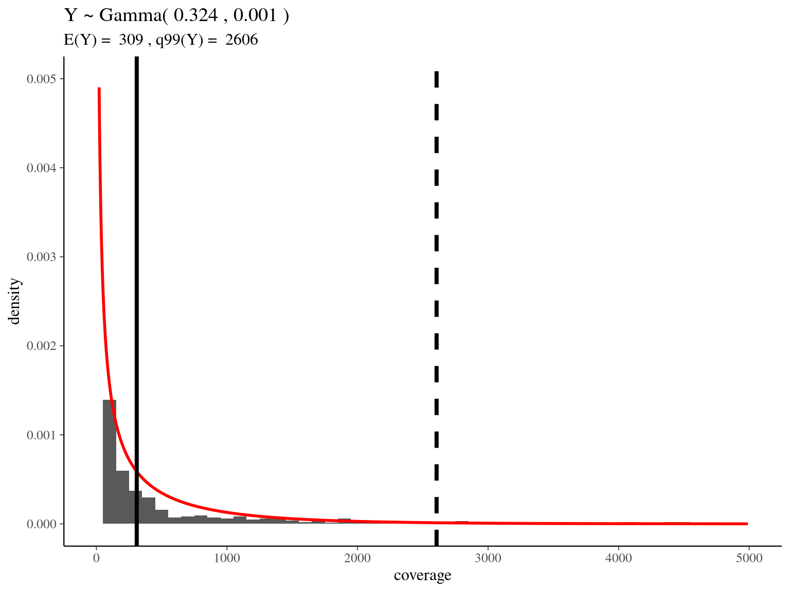
Figure 2.12: Read coverage distribution.
repetitive_target <- bed %>%
  filter(coverage > qgamma(0.99, alpha, beta)) %>%
  mutate(size = end - start)
repetitive_target %>%
  select(target, start, end) %>%
  arrange(target, start, end) %>%
  mutate_if(is.numeric, as.character) %>%
  write_tsv(path = file.path(path, "functional_selection2", "repetitive_targets.bed"),
            col_names = F)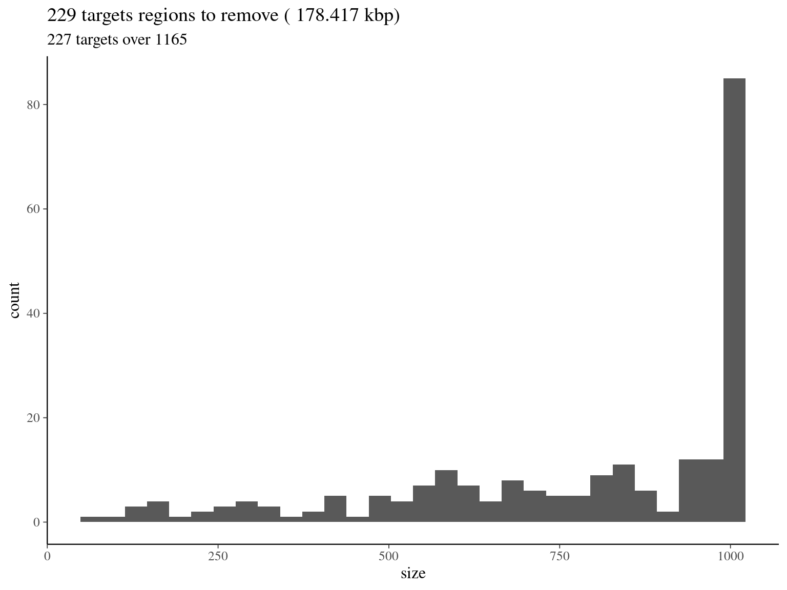
Figure 2.13: target regions with a coverage over the 99th quantile of the fitted Gamma distribution (2606).
cd ~/Documents/BIOGECO/PhD/data/Symphonia_Genomes/functional_selection2
cat repetitive_targets.bed | sort -k 1,1 -k2,2n >  repetitive_targets.sorted.bed
bedtools maskfasta -fi targets.fasta -bed repetitive_targets.sorted.bed -fo targets.masked.fasta
targets <- readDNAStringSet(file.path(path, "functional_selection2", "targets.masked.fasta"))
writeXStringSet(targets[which(letterFrequency(targets, "N")/width(targets) < 0.65)],
file.path(path, "functional_selection2", "targets.filtered.masked.fasta"))| N | Width (Mbp) | Mask (%N) |
|---|---|---|
| 975 | 0.896759 | 0.0168273 |
References
Chakraborty, M., Baldwin-Brown, J.G., Long, A.D. & Emerson, J.J. (2016). Contiguous and accurate de novo assembly of metazoan genomes with modest long read coverage. Nucleic Acids Research, 44, 1–12.
Haas, B.J., Papanicolaou, A., Yassour, M., Grabherr, M., Philip, D., Bowden, J., Couger, M.B., Eccles, D., Li, B., Macmanes, M.D., Ott, M., Orvis, J., Pochet, N., Strozzi, F., Weeks, N., Westerman, R., William, T., Dewey, C.N., Henschel, R., Leduc, R.D., Friedman, N. & Regev, A. (2013). De novo transcript sequence recostruction from RNA-Seq: reference generation and analysis with Trinity.
Kent, W.J. (2002). BLAT—The BLAST-Like Alignment Tool. Genome Research, 12, 656–664.
Li, H. & Durbin, R. (2009). Fast and accurate short read alignment with Burrows-Wheeler transform. Bioinformatics, 25, 1754–1760.
Lopez-Maestre, H., Brinza, L., Marchet, C., Kielbassa, J., Bastien, S., Boutigny, M., Monnin, D., Filali, A.E., Carareto, C.M., Vieira, C., Picard, F., Kremer, N., Vavre, F., Sagot, M.F. & Lacroix, V. (2016). SNP calling from RNA-seq data without a reference genome: Identification, quantification, differential analysis and impact on the protein sequence. Nucleic Acids Research, 44, gkw655. Retrieved from https://academic.oup.com/nar/article-lookup/doi/10.1093/nar/gkw655
Olsson, S., Seoane-Zonjic, P., Bautista, R., Claros, M.G., González-Martínez, S.C., Scotti, I., Scotti-Saintagne, C., Hardy, O.J. & Heuertz, M. (2017). Development of genomic tools in a widespread tropical tree, Symphonia globulifera L.f.: a new low-coverage draft genome, SNP and SSR markers. Molecular Ecology Resources, 17, 614–630. Retrieved from http://doi.wiley.com/10.1111/1755-0998.12605
Smit, A., Hubley, R. & Green, P. (2015). RepeatMasker Open-4.0. <http://www.repeatmasker.org>.