Chapter 6 Neighbourhood crowding effect on neutral and adaptive genetic variation
We did environmental association analyses (Rellstab et al. 2015) in each complex using general linear mixed models developed for genome wide association studies (GWAS). We used the mean neighbourhood crowding index (\(NCI\); Uriarte et al. 2004) over the last 30 years, an indirect measurement of access to light and forest gap dynamics, as the response variable and genetic structure (gene pools representing species) and relatedness (kinship matrix) as explanatory variables, as it is common practice (Rellstab et al. 2015). This analysis assumed that the neighbourhood crowding conditions where individuals have grown above 10-cm DBH are strongly correlated to the individual heritable phenotypes (e.g. Eckert et al. 2010). The mean neighbourhood crowding index \(NCI_i\) from tree individual \(i\) was calculated as follows:
\[NCI_i=\overline{\sum_{j|\delta_{i,j}<20m}DBH^2_{j,t}.e^{-\frac14\delta_{i,j}}}\]
with \(DBH_{j,t}\) the diameter of the neighbouring tree \(j\) in year \(t\) and \(\delta_{i,j}\) its distance to the individual tree \(i\). \(NCI_i\) is computed for all neighbours at a distance \(\delta_{i,j}\) inferior to the maximum neighbouring distance of 20 meters. The power of neighbours \(DBH_{j,t}\) effect was set to 2 to represent a surface. The decrease of neighbours’ diameter effect with distance was set to -0.25 to represent trees at 20 meters of the focal trees having 1% of the effect of the same tree at 0 meters. \(NCI_i\) is computed as the mean of yearly \(NCI_{i,t}\) over the last 30 years denoted by the overline.
We used genetic species and individual kinship in an animal model (Wilson et al. 2010) to estimate genetic variance associated with neighbourhood crowding index.
We used a lognormal likelihood given that distributions of environmental variables were positive and skewed.
We inferred individual kinship using KING (Manichaikul et al. 2010), as the method is robust to population structure.
We set negative kinship values to null as they were confounding with population structure, and we further ensured that the matrix was positive-definite using the nearPD function from the R package Matrix.
The environment \(y_{s,i}\) where individual \(i\) in species \(s\) grows was inferred with a lognormal distribution with the following formula:
\[y_{s,i} \sim logN(log(\mu_s.a_{i}),\sigma^2_1)\] \[a_{i} \sim MVlogN_N(log(1),\sigma^2_2.K)\]
where \(\mu_s\) is the mean environment of species \(s\), \(a_i\) is the breeding value of the individual \(i\) and \(\sigma^2_1\) is the shape parameter of the lognormal.
Individual breeding values \(a_i\) are defined following a multivariate lognormal law \(\mathcal{MVlogN}\) of co-shape matrix defined as the product of the kinship matrix \(K\) with estimated individual genotypic variation \(\sigma^2_2\).
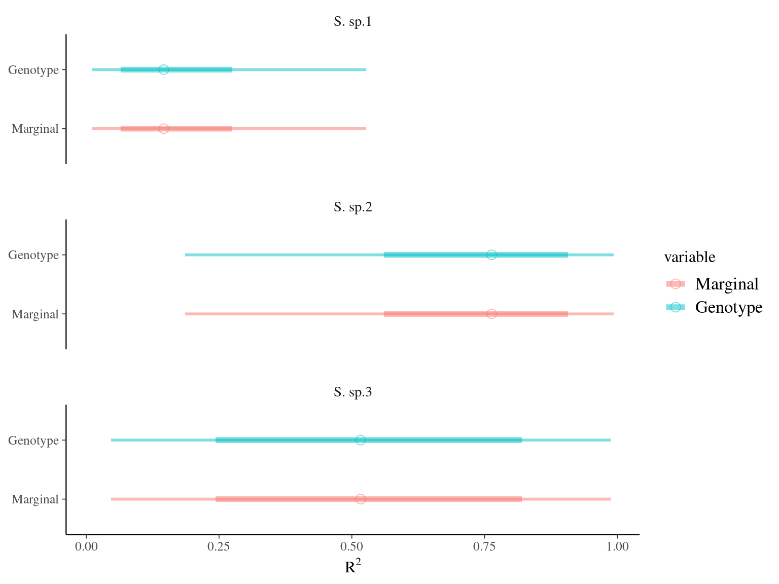
To estimate variances on a normal scale, we log-transformed species fixed effect, genetic additive values, and we calculated conditional and marginal \(R^2\) (Nakagawa & Schielzeth 2013).
A Bayesian method was used to infer parameters using stan language (Carpenter et al. 2017) and the rstan package (Stan Development Team 2018) in the R environment (R Core Team 2020) using the No-U-Turn Sampler algorithm (NUTS, Hoffman & Gelman 2014), which performs better for estimating genetic parameters and breeding values (Nishio & Arakawa 2019).
6.1 Simulated Animal Model
The aim of this subchapter is to explore the animal model with generated data to validate their behaviour and use it on Symphonia real data. Let’s consider a set of \(P=3\) populations including each \(Fam=3\) families composed of \(I = 14\) individuals with arbitrary relationships (it’s only 126 individuals to do quick tests).
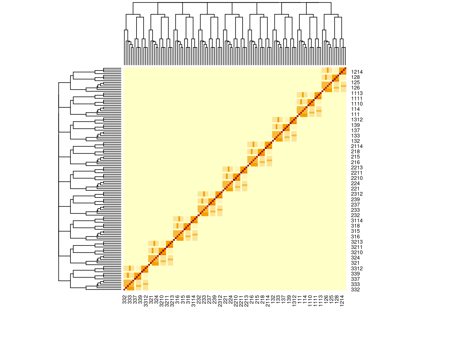
Figure 6.1: Kinship matrix
We used the following animal model with a lognormal distribution to estimate population and genotypic variance:
\[\begin{equation} y_{p,i} \sim \mathcal{logN}(log(\mu_p.a_{i}),\sigma_1) \\ a_{p,i} \sim \mathcal{MVlogN_N}(log(1),\sigma_2.K) \tag{6.1} \end{equation}\]
We fitted the equivalent model with the following priors:
\[\begin{equation} y_{p,i} \sim \mathcal{logN}(log(\mu_p.\hat{a_{i}}), \sigma_1) \\ \hat{a_{i}} = e^{\sqrt{V_G}.A.\epsilon_i} \\ \epsilon_i \sim \mathcal{N}(0,1) \\ ~ \\ \mu_p \sim \mathcal{logN}(log(1),1) \\ \sigma_1 \sim \mathcal N_T(0,1) \\ ~ \\ V_Y = Var(log(y)) \\ V_P = Var(log(\mu_p)) \\ V_R=\sigma_1^2 \\ V_G = V_Y - V_P - V_R \\ \tag{6.2} \end{equation}\]
| Parameter | Estimate | Expected | Standard error | \(\hat R\) |
|---|---|---|---|---|
| mu[1] | 0.7484767 | 0.7357714 | 0.0535640 | 1.0054690 |
| mu[2] | 0.3968538 | 0.3633681 | 0.0308554 | 1.0010121 |
| mu[3] | 0.5184509 | 0.5420625 | 0.0469693 | 1.0023625 |
| Vp | 0.0711053 | 0.0841187 | 0.0151127 | 1.0011662 |
| Vg | 0.0772814 | 0.0837454 | 0.0223466 | 1.0014673 |
| Vr | 0.0385718 | 0.0400000 | 0.0145103 | 0.9997977 |
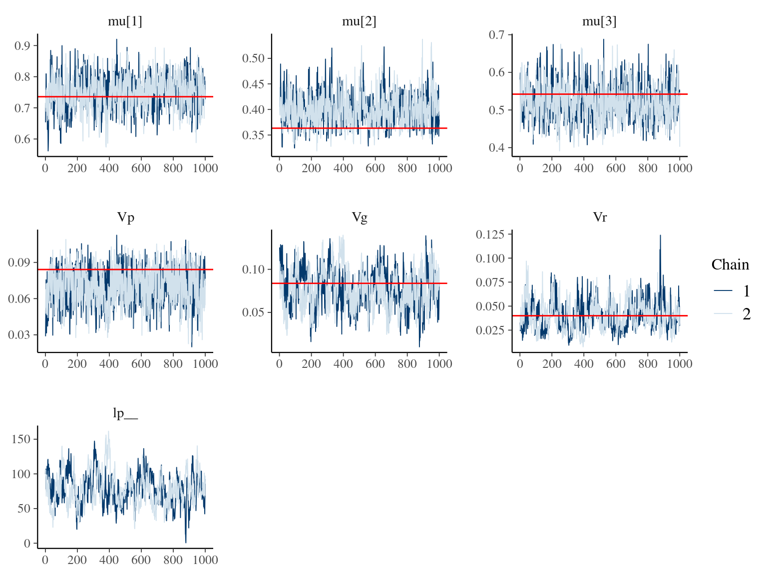
Figure 6.2: Parameters for the Animal model: trace plot and expected value in red.
6.2 Neighbourhood crowding index
trees <- src_sqlite(file.path("data", "Paracou","trees", "Paracou.sqlite")) %>%
  tbl("Paracou") %>%
  filter(Genus == "Symphonia") %>%
  filter(CensusYear == 2015) %>%
  collect()
trees <- read_tsv(file.path(path, "..", "variantCalling", "paracou3pop",
                                                  "symcapture.all.biallelic.snp.filtered.nonmissing.paracou3pop.fam"),
         col_names = c("FID", "IID", "FIID", "MIID", "sex", "phenotype")) %>%
  mutate(Ind = gsub(".g.vcf", "", IID)) %>%
  mutate(X = gsub("P", "", Ind)) %>%
  separate(X, c("Plot", "SubPlot", "TreeFieldNum"), convert = T) %>%
  left_join(trees) %>%
  left_join(read_tsv(file.path(path, "bayescenv", "paracou3pop.popmap"),
                     col_names = c("IID", "pop")))
cl <- parallel::makeCluster(getOption("cl.cores", 4))
parallel::clusterExport(cl, list("trees"))
NC <- parallel::parLapply(cl, 1:nrow(trees), function(ind){
  library(tidyverse)
  src_sqlite(file.path("data", "Paracou", "trees", "Paracou.sqlite")) %>%
    tbl("Paracou") %>%
    filter(Plot == local(trees$Plot[ind])) %>%
    filter(idTree != local(trees$idTree[ind])) %>%
    mutate(dij = sqrt((local(trees$Xutm[ind]) - Xutm)^2+(local(trees$Yutm[ind]) - Yutm)^2)) %>%
    filter(dij < 20) %>%
    mutate(con = ifelse(Genus == local(trees$Genus[ind]) && Species == local(trees$Species[ind]), 1, 0)) %>%
    mutate(DBH = CircCorr/pi) %>%
    collect() %>%
    group_by(CensusYear) %>%
    summarise(NCI = sum(DBH*DBH*exp(-0.25*dij))) %>%
    ungroup() %>%
    summarise(idTree = local(trees$idTree[ind]),
              NCI = mean(NCI))})
parallel::stopCluster(cl) ; rm(cl)
NC <- bind_rows(NC)
trees <- left_join(trees, NC) %>%
  dplyr::select(IID, Ind, pop, NCI)
rm(NC)
write_tsv(trees, file = "save/NCI.tsv")
6.3 Genetic variance
We used between individual kinship and a lognormal Animal model (Wilson et al. 2010) to estimate genetic variance associated to individuals’ global phenotype living in a given environment (see environmental association analyses with genome wide association study analyses in Rellstab et al. 2015). The animal model is calculated for the environmental values \(y\) of the \(N\) individuals with the following formula:
\[\begin{equation} y_{p,i} \sim \mathcal{logN}(log(a_{p,i}),\sigma_1) \\ a_{p,i} \sim \mathcal{MVlogN_N}(log(\mu_p),\sigma_2.K) \tag{6.3} \end{equation}\]
where individual is defined as a normal law centered on the individual genetic additive effects \(a\) and associated individual remaining variance \(\sigma_R\). Additive genetic variance \(a\) follows a multivariate lognormal law centered on the population mean \(\mu_{Population}\) of covariance \(\sigma_G K\).
We fitted the equivalent model with following priors:
\[\begin{equation} y_{p,i} \sim \mathcal{logN}(log(\mu_p) + \hat{\sigma_2}.A.\epsilon_i, \sigma_1) \\ \epsilon_i \sim \mathcal{N}(0,1) \\ ~ \\ \mu_p \sim \mathcal{logN}(log(1),1) \\ \sigma_1 \sim \mathcal N_T(0,1) \\ \hat{\sigma_2} = \sqrt(V_G) ~ \\ V_Y = Var(log(y)) \\ V_P = Var(log(\mu_p)) \\ V_G = V_Y - V_P - V_R \\ V_R=\sigma_1^2 \tag{6.4} \end{equation}\]
| Variable | Parameter | Species | Estimate | \(\sigma\) | \(\hat{R}\) |
|---|---|---|---|---|---|
| NCI | mu | S. globulifera Paracou | 0.7880048 | 0.0305778 | 0.9997771 |
| NCI | mu | S. globulifera Regina | 0.9443492 | 0.0643210 | 1.0003822 |
| NCI | mu | S. sp1 | 0.9426952 | 0.0290419 | 1.0012267 |
| NCI | Vp | 0.0071862 | 0.0033377 | 1.0004033 | |
| NCI | Vg | 0.0210950 | 0.0193455 | 1.0640539 | |
| NCI | Vr | 0.0922548 | 0.0193773 | 1.0615180 |
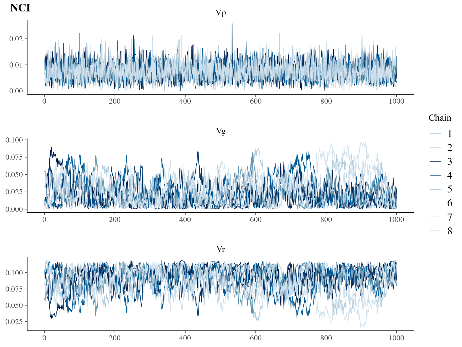
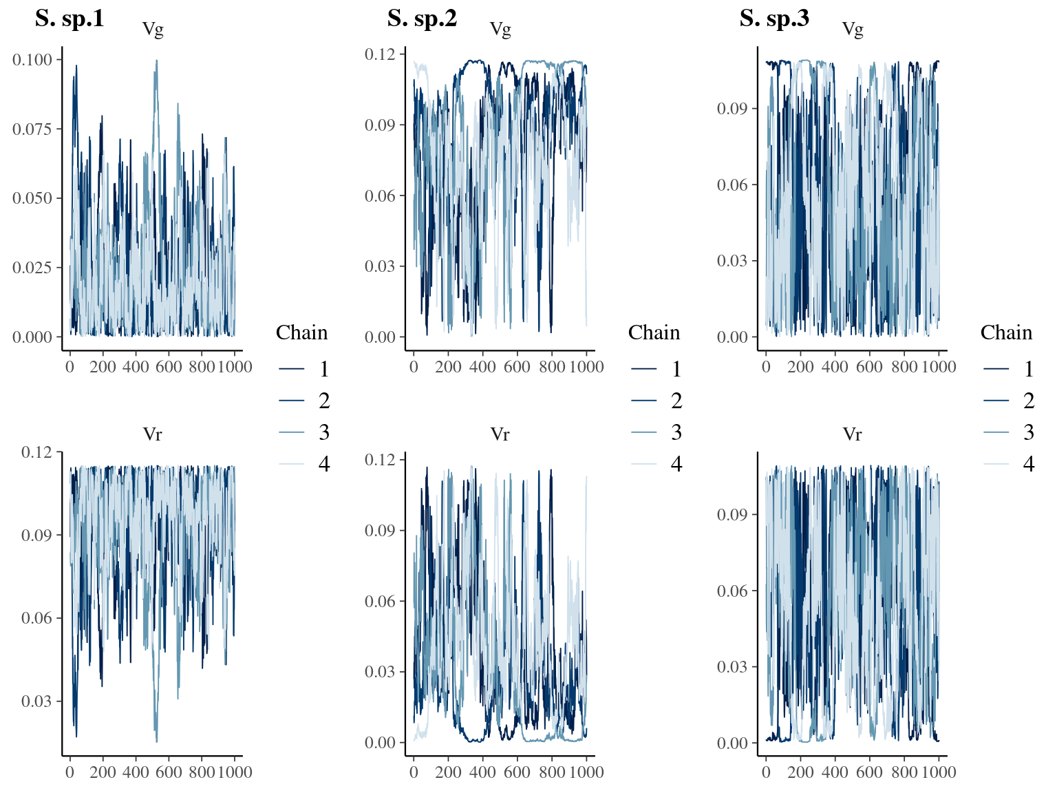
Figure 6.3: Traceplot for environmental variables.
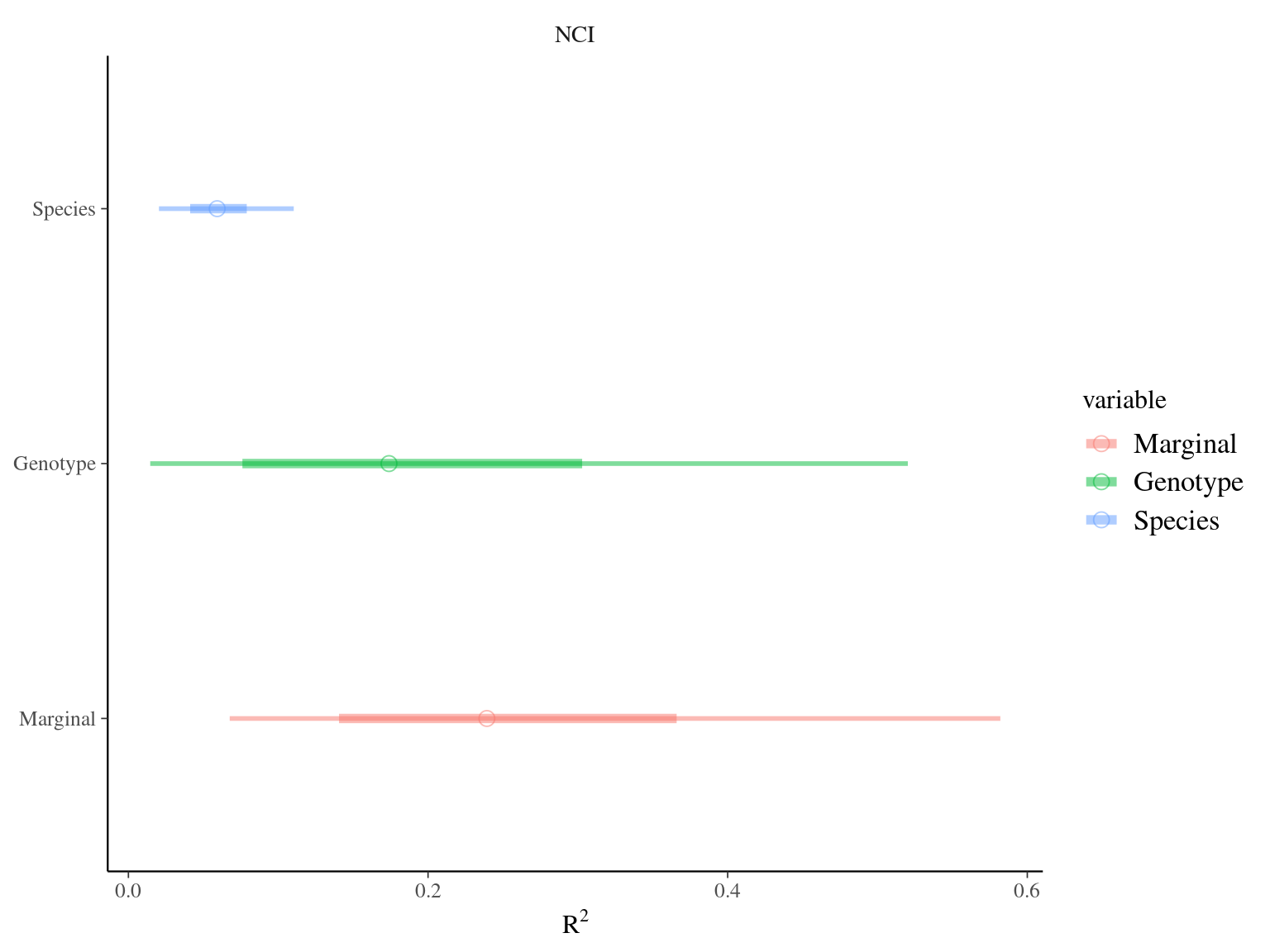
Figure 6.4: R2 for environmental variable
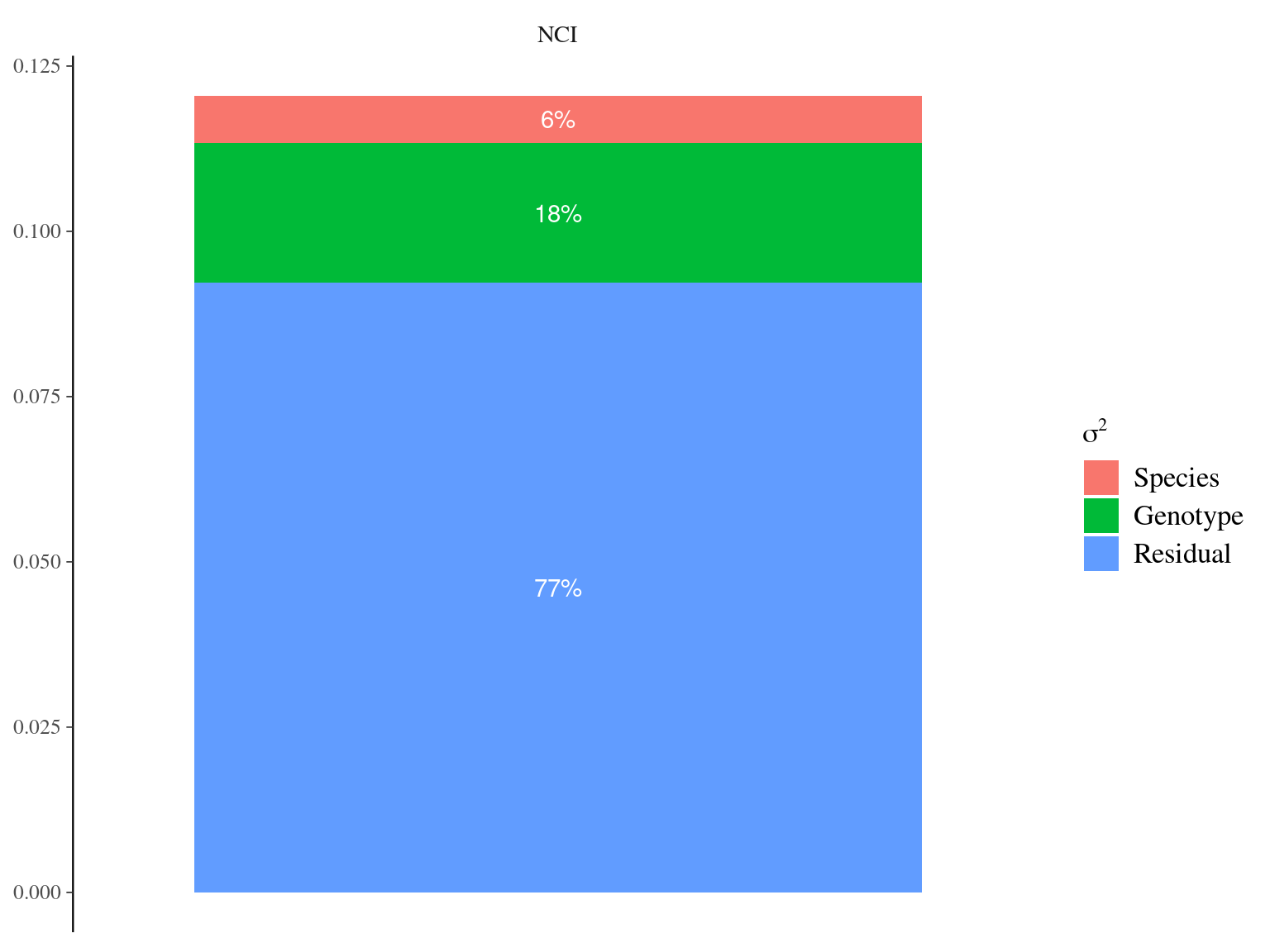
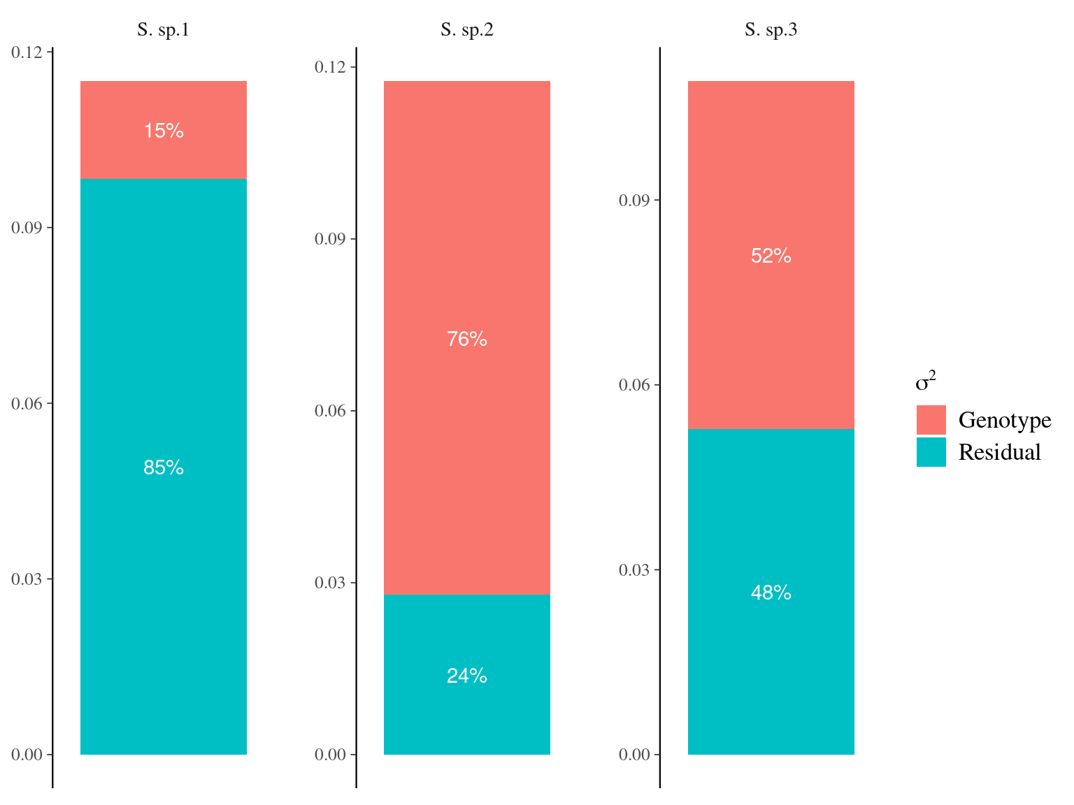
Figure 6.5: Genetic variance partitioning for environmental variables.
6.4 Confounding neutral variation
If the observed genetic variation in relation to the environment is non-adaptive, i.e. confounded by neutral processes, the observed patterns should not differ from the randomized environmental maps across the study plots (Fig. 6.6), preserving the spatial structure of individuals while breaking their relationship with the environment. Instead, we observed a pattern significantly (P < XXX, Fig. ??) different from the patterns observed randomizing environmental maps across plots. Thus, the relationship is adaptive, not neutral.
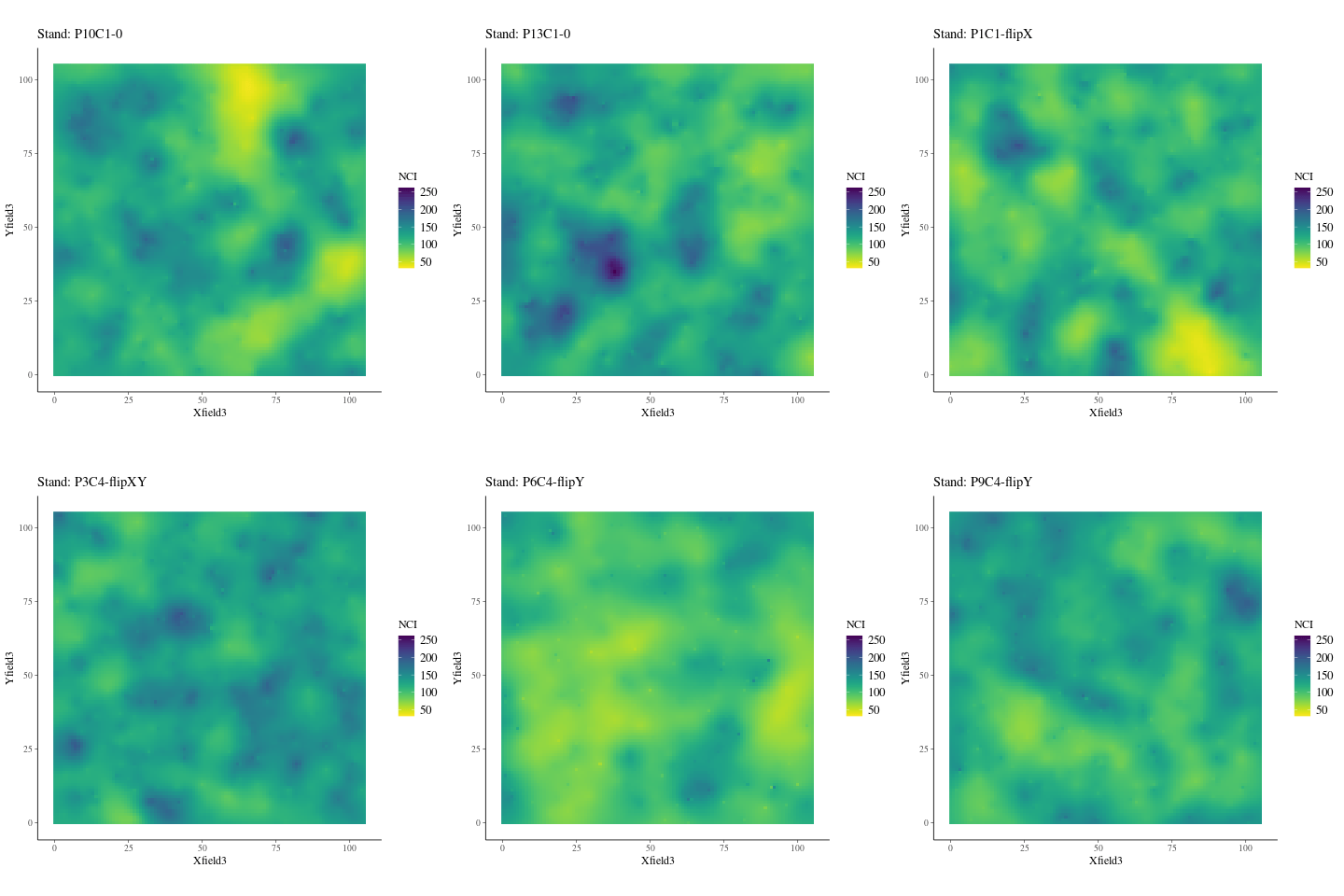
Figure 6.6: NCI in 2015 across SubPlots.
## Error in ss[, !colnames(ss) %in% drop.pars, drop = FALSE] :
##   nombre de dimensions incorrect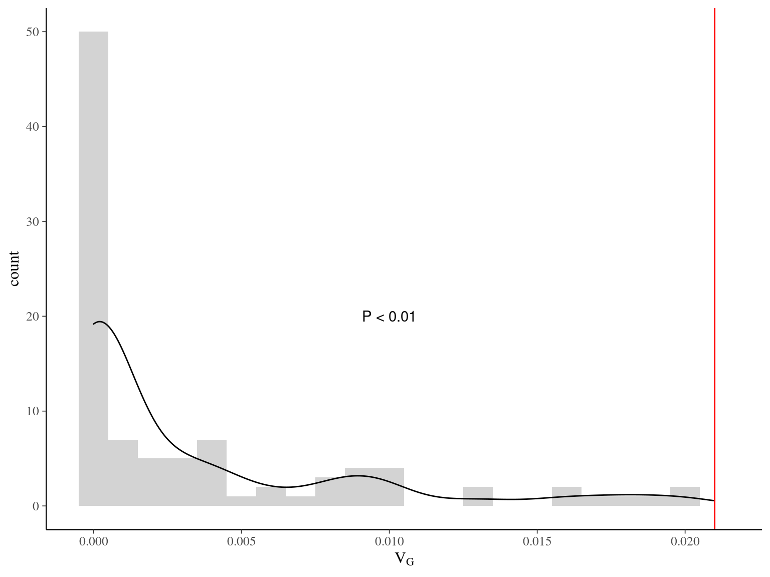
Figure 6.7: Among-genotype variance (VG) between observed value (red) and values observed in null models (black) randomizing neighbourhood crowding index (NCI) among plots.
References
Carpenter, B., Gelman, A., Hoffman, M.D., Lee, D., Goodrich, B., Betancourt, M., Brubaker, M., Guo, J., Li, P. & Riddell, A. (2017). Stan : A Probabilistic Programming Language. Journal of Statistical Software, 76. Retrieved from http://www.jstatsoft.org/v76/i01/
Eckert, A.J., Van Heerwaarden, J., Wegrzyn, J.L., Nelson, C.D., Ross-Ibarra, J., González-Martínez, S.C. & Neale, D.B. (2010). Patterns of population structure and environmental associations to aridity across the range of loblolly pine (Pinus taeda L., Pinaceae). Genetics, 185, 969–982.
Hoffman, M.D. & Gelman, A. (2014). The no-U-turn sampler: Adaptively setting path lengths in Hamiltonian Monte Carlo. Journal of Machine Learning Research, 15, 1593–1623. Retrieved from http://arxiv.org/abs/1111.4246
Manichaikul, A., Mychaleckyj, J.C., Rich, S.S., Daly, K., Sale, M. & Chen, W.M. (2010). Robust relationship inference in genome-wide association studies. Bioinformatics, 26, 2867–2873.
Nakagawa, S. & Schielzeth, H. (2013). A general and simple method for obtaining R2 from generalized linear mixed-effects models. Methods in Ecology and Evolution, 4, 133–142.
Nishio, M. & Arakawa, A. (2019). Performance of Hamiltonian Monte Carlo and No-U-Turn Sampler for estimating genetic parameters and breeding values. Genetics Selection Evolution, 51, 1–12. Retrieved from https://doi.org/10.1186/s12711-019-0515-1
R Core Team. (2020). R: A Language and Environment for Statistical Computing.
Rellstab, C., Gugerli, F., Eckert, A.J., Hancock, A.M. & Holderegger, R. (2015). A practical guide to environmental association analysis in landscape genomics. 24, 4348–4370. Retrieved from http://doi.wiley.com/10.1111/mec.13322
Stan Development Team. (2018). Rstan: the R interface to Stan. Retrieved from http://mc-stan.org/
Uriarte, M., Condit, R., Canham, C.D. & Hubbell, S.P. (2004). A spatially explicit model of sapling growth in a tropical forest: Does the identity of neighbours matter? Journal of Ecology, 92, 348–360. Retrieved from http://doi.wiley.com/10.1111/j.0022-0477.2004.00867.x
Wilson, A.J., Réale, D., Clements, M.N., Morrissey, M.M., Postma, E., Walling, C.A., Kruuk, L.E.B. & Nussey, D.H. (2010). An ecologist’s guide to the animal model. Journal of Animal Ecology, 79, 13–26. Retrieved from https://pdfs.semanticscholar.org/931b/921e07dc932e3f34e78bc3ca5a7bfe472e04.pdf
