Chapter 5 Genetic species delimitation

We investigated population genetic structure using admixture (Alexander & Lange 2011), using 10 repetitions of K genetic groups varying from 1 to 10 and assessed the number of gene pools with cross validation. We defined individuals with a membership to gene pools below 90% as admixed and the remaining individuals as genetically pure. We further investigated admixture with the introgress R package (Gompert & Alex Buerkle 2010), using genetically pure individuals as parental populations and all individuals as the hybrid population. We validated gene pool delimitation by comparison with botanical identifications using a confusion matrix, and we conducted a second blind-identification of every collected individual in November 2019.

5.1 Populations structure

Symphonia individuals were structured in three gene pools in Paracou corresponding to field morphotypes (Fig. 5.1 and Fig. 5.2). The three genotypes correspond to the previously identified two morphotypes (70-80%) S. globulifera and S. sp1, with S. globulifera morphotype structured in two gene pools, which might match the two identified sub-morphotype in Paracou called S. globulifera type Paracou (80%) and S. globulifera type Régina (20%). Interestingly, we noticed the so-called Paracou type and Régina type within S. globulifera morphotype when sampling the individuals. And looking at a few identified individuals’ bark, the two identified gene pools correspond two these two morphotypes (Fig. 5.5). The Paracou type has a smoother and thinner bark compared to the thick and lashed bark of the Régina type.

module load bioinfo/admixture_linux-1.3.0
module load bioinfo/plink-v1.90b5.3
mkdir admixture
mkdir admixture/paracou
mkdir out
cd ../variantCalling
mkdir paracouRenamed
# read_tsv(file.path(pathCluster, "paracou", "symcapture.all.biallelic.snp.filtered.nonmissing.paracou.bim"),
#          col_names = F) %>% 
#   mutate(X1 = as.numeric(as.factor(X1))) %>% 
#   write_tsv(file.path(pathCluster, "paracouRenamed", "symcapture.all.biallelic.snp.filtered.nonmissing.paracou.bim"),
#             col_names = F)
cp paracou/symcapture.all.biallelic.snp.filtered.nonmissing.paracou.bed paracouRenamed
cp paracou/symcapture.all.biallelic.snp.filtered.nonmissing.paracou.fam paracouRenamed 
cd ../populationGenomics/admixture/paracou
for k in $(seq 10) ; do echo "module load bioinfo/admixture_linux-1.3.0 ; admixture --cv ../../variantCalling/paracouRenamed/symcapture.all.biallelic.snp.filtered.nonmissing.paracou.bed $k | tee log$k.out" ; done > admixture.sh
sarray -J admixture -o ../../out/%j.admixture.out -e ../../out/%j.admixture.err -t 48:00:00 --mem=8G --mail-type=BEGIN,END,FAIL admixture.sh
scp sschmitt@genologin.toulouse.inra.fr:~/Symcapture/populationGenomics/admixture/paracou/*
grep -h CV log*.out > CV.out
for file in $(ls log*.out) ; do  grep "Fst divergences between estimated populations:" -A 20 $file | head -n -2 > matrices/$file ; done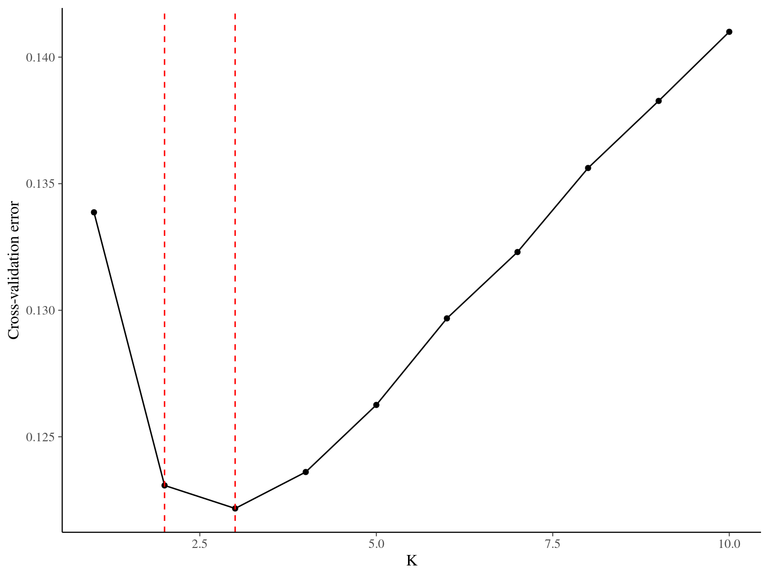

Figure 5.1: Cross-validation for the clustering of Paracou individuals. Y axis indicates cross-validation mean error, suggesting that 2 or 3 groups best represent the genetic structure of individuals in Paracou.

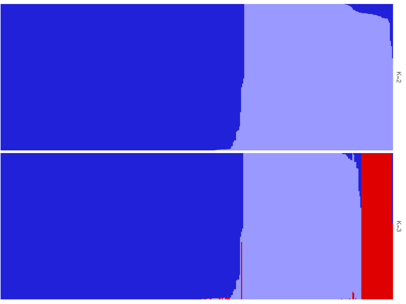
Figure 5.2: Population structure of Paracou individuals for K=2 and K=3. Dark blue is associated with S. globulifera morphotype; whereas light blue is associated with S. sp1; and red is associated with a subgroup within the S. globulifera morphotype.

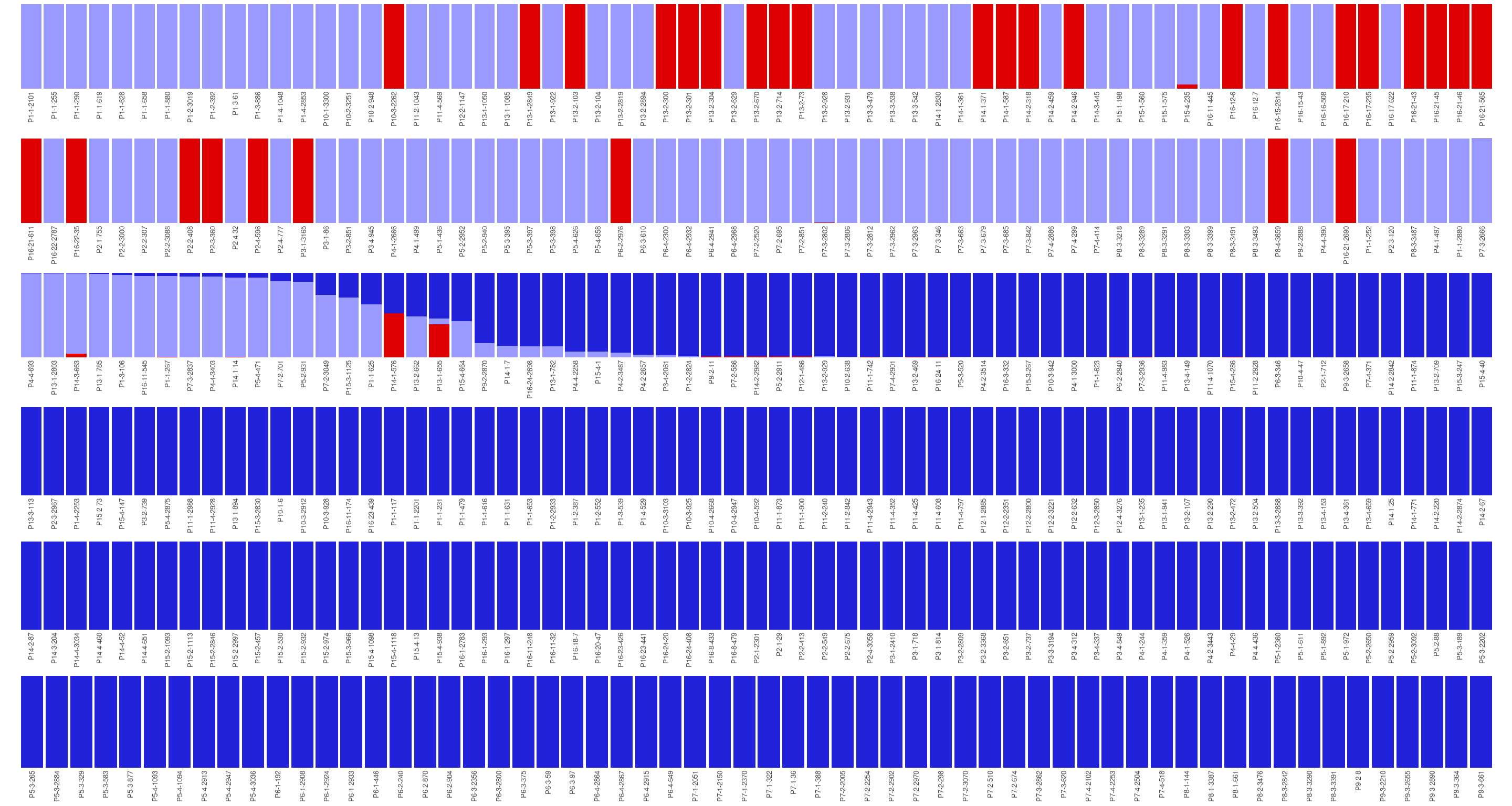
Figure 5.3: Population structure of Paracou individuals for K = 2. Dark blue is associated with the S. globulifera morphotype; whereas light blue is associated with S. sp1

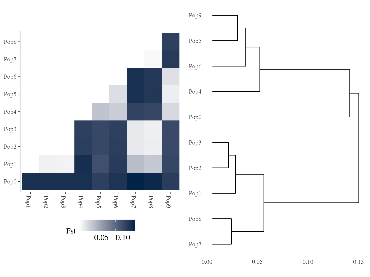
Figure 5.4: Clusters Fst relations for K=10.

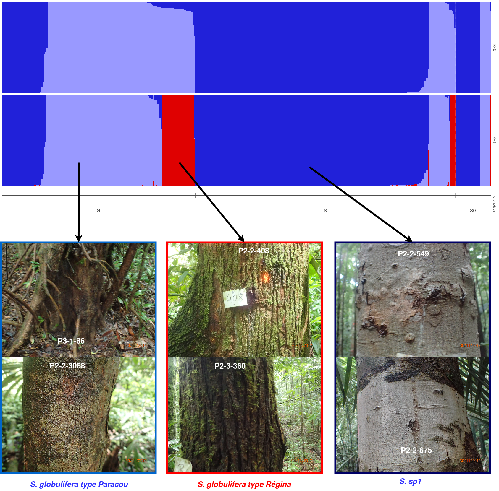
Figure 5.5: The Symphonia globulifera morphotypes identified in the field. The three morphotypes are identified with their bark with S. sp1 having a light grey thin and smooth bark, the S. globulifera type Paracou having a dark and intermediate thin and smooth bark compared to the thick and lashed bark of S. globulifera type Regina.

5.2 Kinship

We calculated kinship matrix for every individual to be used in a genomic scan to control for population structure. 19 individuals, belonging to all gene pools, had only negative kinship values. After investigation it seems that these individuals are individuals without family in Paracou with null kinship with other individuals of their gene pools and negative values with other individuals of other gene pools. Interestingly though, individuals with only null or negative kinship were all located on the limit of Paracou plots.

module load bioinfo/plink-v1.90b5.3
plink \
  --bfile symcapture.all.biallelic.snp.filtered.nonmissing.paracou \
  --allow-extra-chr \
  --recode vcf-iid \
  --out symcapture.all.biallelic.snp.filtered.nonmissing.paracou
vcftools --gzvcf  symcapture.all.biallelic.snp.filtered.nonmissing.paracou.vcf.gz  --relatedness2
# an estimated kinship coefficient range >0.354, [0.177, 0.354], [0.0884, 0.177] and [0.0442, 0.0884] corresponds to duplicate/MZ twin, 1st-degree, 2nd-degree, and 3rd-degree relationships respectively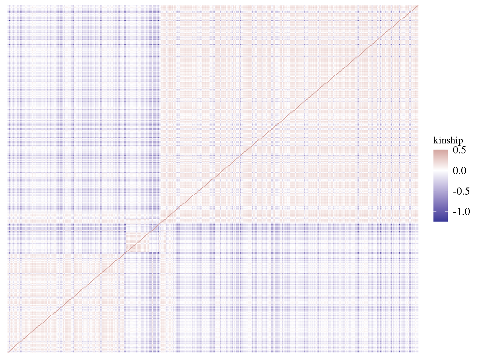

Figure 5.6: Individuals kinship matrix.

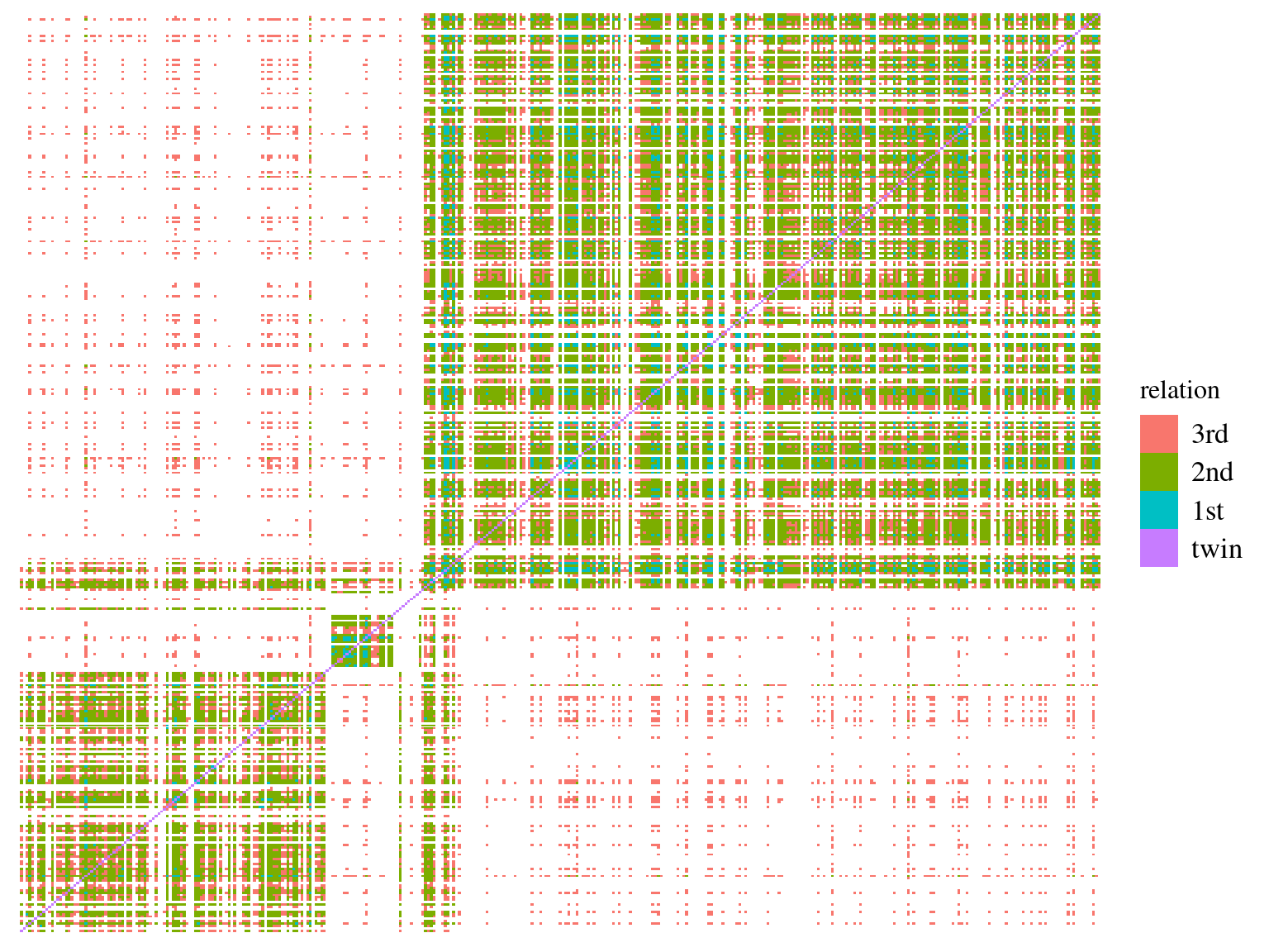
Figure 5.7: Individuals kinship matrix.

5.3 Spatial auto-correlation

plink=~/Tools/plink_linux_x86_64_20190617/plink 
$plink \
  --bfile ../paracou/symcapture.all.biallelic.snp.filtered.nonmissing.paracou \
  --allow-extra-chr \
  --keep sp1.fam \
  --recode vcf-iid \
  --thin-count 1000 \
  --out sp1.1k

snps <- vroom::vroom(file.path(path, "..", "variantCalling", "spagedi", "globuliferaTypeRegina.1k.genepop"), skip = 1002, 
                     col_names = c("Lib", "Lat", "Long", paste0("SNP", 1:1000)))
XY <- mutate(snps, Ind = gsub(".g.vcf", "", Lib)) %>% 
  dplyr::select(Ind) %>% 
  left_join(dplyr::select(trees, Ind, Xutm, Yutm))
snps$Lat <- XY$Xutm
snps$Long <- XY$Yutm
write_tsv(snps, path = file.path(path, "..", "variantCalling", "spagedi", "globuliferaTypeRegina.1k.spagedi.in"), col_names = T)

// #ind #cat #coord #loci #dig/loc #ploidy// this an example (lines beginning by // are comment lines)
231 0   2   1000    3   2
8   25  50  100 200 400 800 1600 3200

spagedi
sp1.1k.spagedi.in  
sp1.1k.spagedi.out
e
return
13
3
return
1000
34
3

Locus intra-individual (inbreeding coef) 1 2 3 4 5 6 7 average 0-2704.88 b-lin(slope linear dist) b-log(slope log dist) ALL LOCI -0.0480 0.0079 0.0049 0.0046 0.0036 0.0035 0.0023 -0.0001 0.0001 -1.34448E-06 -0.00128963 F F1 F2 b-log Sp = –b-log / (1 − F1)

## [1] "S. sp.1 Sp = 0.000458510425020048"

## [1] "S. sp.2 Sp = 0.00110720539398209"

## [1] "S. sp.3 Sp = 0.000132259359630633"

5.4 Environmental auto-correlation

trees <- read_tsv(file = "save/NCI.tsv") 
snps <- vroom::vroom(file.path(path, "..", "variantCalling", "spagedienv", "sp2.1k.genepop"), skip = 1002, 
                     col_names = c("Lib", "nci", "Long", paste0("SNP", 1:1000))) %>% 
  dplyr::select(-Long)
NCI <- mutate(snps, Ind = gsub(".g.vcf", "", Lib)) %>% 
  dplyr::select(Ind) %>% 
  left_join(dplyr::select(trees, Ind, NCI))
snps$nci <- NCI$NCI
write_tsv(snps, path = file.path(path, "..", "variantCalling", "spagedienv", "sp2.1k.spagedi.in"), col_names = T)

// #ind #cat #coord #loci #dig/loc #ploidy// this an example (lines beginning by // are comment lines)
30  0   1   1000    3   2
-8


spagedi
sp1.1k.spagedi.in  
sp1.1k.spagedi.out
e
return
13
3
return
1000
34
3

## [1] "S. sp.1 Sp = 0.000458510425020048"

## [1] "S. sp.2 Sp = 0.00110720539398209"

## [1] "S. sp.3 Sp = 0.000206395606617702"

5.5 Introgression

We used the method developed by Gompert & Buerkle (2009) implemented in introgress (Gompert & Alex Buerkle 2010) to map admixture between Paracou genepools. We used individuals with more than 90% of the genotype belonging to the genepool to define parental allele frequencies and mapped admixture between the two pairs of S. sp1 - S. globulifera Paracou and S. sp1 - S. globulifera Regina as the remaining pair didn’t show any admixture signs with the admixture software. We furthered classified individuals as (i) pure-bred with a hybrid index \(h\) above 0.9, (ii) introgressed with \(h \in [0.6-0.9]\), and (iii) admixed with \(h \in [0.5-0.6]\).

We obtained relatively low levels of admixture (Fig. 5.8) with 222 S. sp1 pure-bred, 108 S. globulifera Paracou pure-bred, and 30 S. globulifera Regina pure-bred. Only 5 individuals were admixed (2 S. sp1 - S. globulifera Regina and 3 S. sp1 - S. globulifera Paracou). Nevertheless S. sp1 showed 13(6%) individuals introgressed with S. globulifera Regina and S. globulifera Paracou showed 7(6%) individuals introgressed with S. sp1.

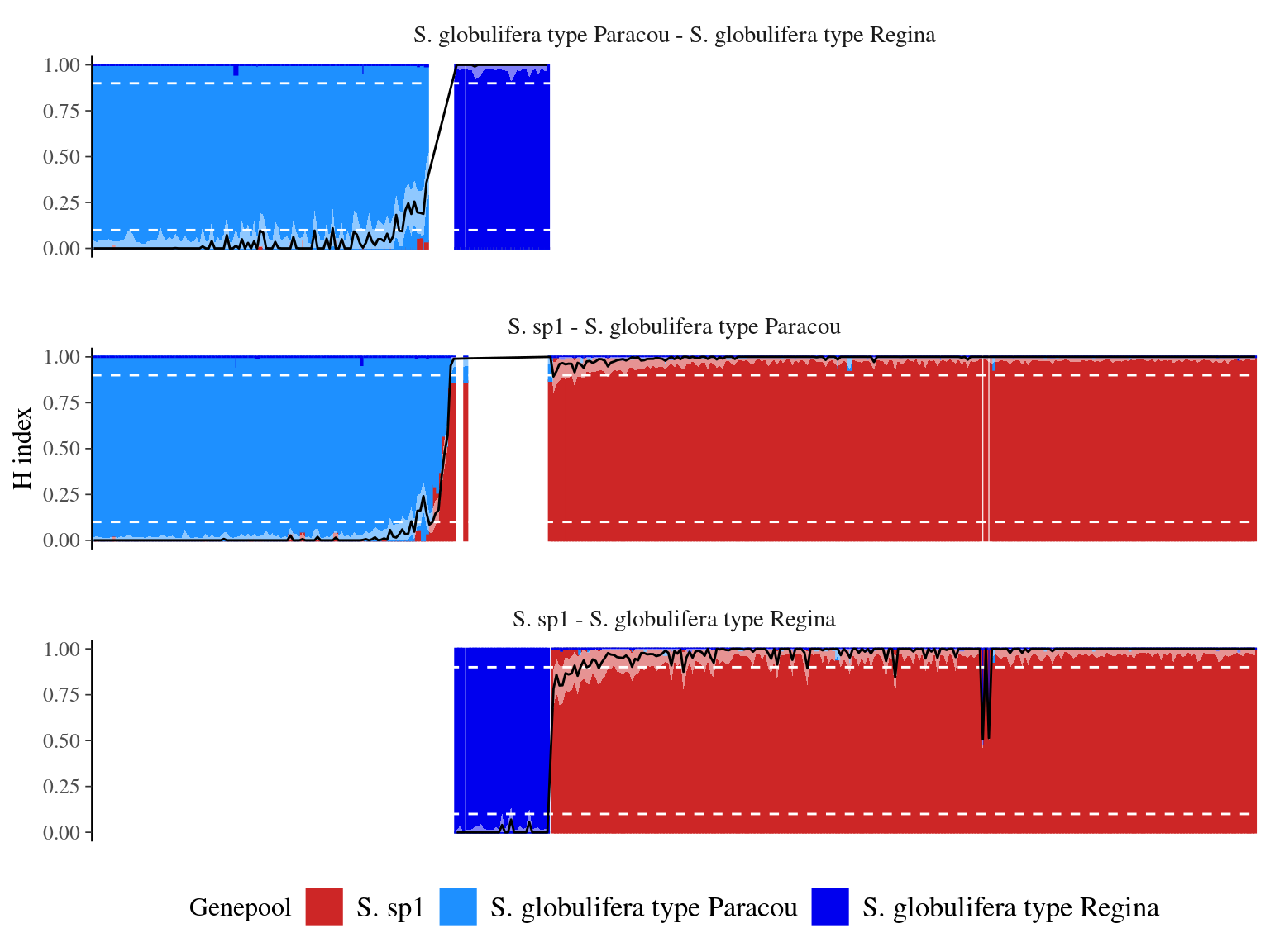
Figure 5.8: Population structure and fraction of the genome inherited from S. sp1 for each individual (hybrid index or admixture coefficient). Population structure assessed with ADMIXTURE is represented with the color bar for each individual, with the percentage of membership to the S. sp1 gene pool represented by the bar height. The hybrid index and it’s confidence interval is represented by the black line and the white area. The white dashed line indicates levels used to define previous gene pools and parental alleles frequencies.

References

Alexander, D.H. & Lange, K. (2011). Enhancements to the ADMIXTURE algorithm for individual ancestry estimation. BMC Bioinformatics, 12.

Gompert, Z. & Alex Buerkle, C. (2010). Introgress: A software package for mapping components of isolation in hybrids. Molecular Ecology Resources, 10, 378–384.

Gompert, Z. & Buerkle, C.A. (2009). A powerful regression-based method for admixture mapping of isolation across the genome of hybrids. Molecular Ecology, 18, 1207–1224.