Chapter 7 Neutral and adaptive genetic variation effect on individual growth
We investigated effects of ecological and evolutionary processes on individual growth, using genetic species and kinship. The individual growth of individual \(i\) in population \(p\) between individual recruitment \(y_0\) and 2017, corresponds to the difference of DBH between the two years, and is defined with a hierarchical model in a lognormal distribution as follows:
\[DBH_{y=2017,p,i} - DBH_{y=y0,p,i} \sim logN(log[\sum_{y=y0}^{y=2017}AGR(DBH_{y,p,i})], \sigma^2_1)\]
where the difference of DBH \(DBH_{y=2017,p,i}-DBH_{y=y_0,p,i}\) is defined with a lognormal distribution located on the logarithm of the sum of annual growth rates \(AGR\) during the period \(y_0-2017\) and of shape \(\sigma_1\). The annual growth rate \(AGR\) for individual \(i\) in population \(p\) at year \(y\) with a diameter of \(DBH_{y,p,i}\) is defined following a Gompertz model (Gompertz 1825) already identified as the best model for growth-trajectories in Paracou (Hérault et al. 2011):
\[AGR(DBH_{y,p,i}) = Gmax_i.exp(-\frac12[\frac{log(\frac{DBH_{y,p,i}}{Doptp})}{Ksp}]^2)\]
where \(Gmax_i\) is the maximum growth potential (maximal AGR during individual life) for individual \(i\), \(Dopt_p\) is the population optimal diameter at which the individual reaches its maximum growth potential, and \(Ks_p\) is the population kurtosis defining the width of the bell-shaped growth-trajectory (see figure 1 in Hérault et al. 2011). To ease model inference, population optimal diameter \(Dopt_p\) and kurtosis \(Ks_p\) were defined as random population effects centered on a global \(Dopt\) and \(Ks\) with corresponding variances \(\sigma^2_{P,Dopt}\) and \(\sigma^2_{P,Ks}\). Individual \(i\) maximum growth potential \(Gmax_i\) was defined in a nested Animal model with a lognormal distribution:
\[Gmax_i \sim logN(log(Gmax_p.a_i), \sigma_{R,Gmax})\] \[a_i \sim MVlogN(log(1), \sigma_{G,Gmax}.K)\]
where \(Gmax_p\) is the mean \(Gmax\) of population \(p\),
\(a_i\) is the breeding value of individual \(i\),
and \(\sigma_{R,Gmax}\) is the shape of the lognormal distribution.
Individual breeding values \(a_i\) are defined following a multivariate lognormal law \(MVlogN\)
with a co-shape matrix defined as the product of the kinship matrix \(K\) and the genotypic variation \(\sigma_{G,Gmax}\).
To estimate variances on a normal-scale, we log-transformed population fixed effect, genetic additive values,
and calculated conditional and marginal \(R^2\) (Nakagawa & Schielzeth 2013).
We used Bayesian inference with No-U-Turn Sampler (NUTS, Hoffman & Gelman 2014) using stan language (Carpenter et al. 2017).
7.1 Growth data
trees <- src_sqlite(file.path("data", "Paracou","trees", "Paracou.sqlite")) %>%
  tbl("Paracou") %>%
  filter(Genus == "Symphonia") %>%
  mutate(DBH = CircCorr/pi) %>%
  filter(!(CodeMeas %in% c(4))) %>%
  collect()
trees <- read_tsv(file.path(path, "..", "variantCalling", "paracou",
                          "symcapture.all.biallelic.snp.filtered.nonmissing.paracou.fam"),
         col_names = c("FID", "IID", "FIID", "MIID", "sex", "phenotype")) %>%
  mutate(Ind = gsub(".g.vcf", "", IID)) %>%
  mutate(X = gsub("P", "", Ind)) %>%
  separate(X, c("Plot", "SubPlot", "TreeFieldNum"), convert = T) %>%
  left_join(trees) %>%
  left_join(read_tsv(file.path(path, "bayescenv", "paracou3pop.popmap"),
                     col_names = c("IID", "pop"))) %>%
  left_join(read_tsv(file.path(path, "populations", "paracou.hybridmap")),
            by = "Ind", suffix = c("", ".hybrid"))
trees <- trees %>%
  group_by(Ind) %>%
  mutate(Y0 = dplyr::first(CensusYear), DBH0 = dplyr::first(DBH),
         DBHtoday = dplyr::last(DBH), N = n()) %>%
  ungroup() %>%
  dplyr::select(Ind, Xutm, Yutm, IID, pop, Y0, DBH0, DBHtoday, N) %>%
  unique() %>%
  mutate(DBHtoday = ifelse(DBHtoday == DBH0, DBHtoday + 0.1, DBHtoday))
write_tsv(trees, file = "save/Growth.tsv")
7.2 Simulated Growth and Animal Model
We used the following growth model with a lognormal distribution to estimate individual growth potential and associated genotypic variation:
\[\begin{equation} DBH_{y=today,p,i} - DBH_{y=y0,p,i} \sim \\ \mathcal{logN} (log(\sum _{y=y_0} ^{y=today} \theta_{1,p,i}.exp(-\frac12.[\frac{log(\frac{DBH_{y,p,i}}{100.\theta_{2,p}})}{\theta_{3,p}}]^2)), \sigma_1) \\ \theta_{1,p,i} \sim \mathcal {logN}(log(\theta_{1,p}.a_{1,i}), \sigma_2) \\ \theta_{2,p} \sim \mathcal {logN}(log(\theta_2),\sigma_3) \\ \theta_{3,p} \sim \mathcal {logN}(log(\theta_3),\sigma_4) \\ a_{1,i} \sim \mathcal{MVlogN}(log(1), \sigma_5.K) \tag{7.1} \end{equation}\]
We fitted the equivalent model with the following priors:
\[\begin{equation} DBH_{y=today,p,i} - DBH_{y=y0,p,i} \sim \\ \mathcal{logN} (log(\sum _{y=y_0} ^{y=today} \hat{\theta_{1,p,i}}.exp(-\frac12.[\frac{log(\frac{DBH_{y,p,i}}{100.\hat{\theta_{2,p}}})}{\hat{\theta_{3,p}}}]^2)), \sigma_1) \\ \hat{\theta_{1,p,i}} = e^{log(\theta_{1,p}.\hat{a_{1,i}}) + \sigma_2.\epsilon_{1,i}} \\ \hat{\theta_{2,p}} = e^{log(\theta_2) + \sigma_3.\epsilon_{2,p}} \\ \hat{\theta_{3,p}} = e^{log(\theta_3) + \sigma_4.\epsilon_{3,p}} \\ \hat{a_{1,i}} = e^{\sigma_5.A.\epsilon_{4,i}} \\ \epsilon_{1,i} \sim \mathcal{N}(0,1) \\ \epsilon_{2,p} \sim \mathcal{N}(0,1) \\ \epsilon_{3,p} \sim \mathcal{N}(0,1) \\ \epsilon_{4,i} \sim \mathcal{N}(0,1) \\ ~ \\ (\theta_{1,p}, \theta_2, \theta_3) \sim \mathcal{logN}^3(log(1),1) \\ (\sigma_1, \sigma_2, \sigma_3, \sigma_4, \sigma_5) \sim \mathcal{N}^5_T(0,1) \\ ~ \\ V_P = Var(log(\mu_p)) \\ V_G=\sigma_5^2\\ V_R=\sigma_2^2 \tag{7.2} \end{equation}\]
| Parameter | Estimate | Standard error | Expected | \(\hat R\) |
|---|---|---|---|---|
| thetap1[1] | 0.8266180 | 0.1121729 | 0.5300000 | 1.0008119 |
| thetap1[2] | 0.4816256 | 0.0889950 | 0.5400000 | 1.0015447 |
| thetap1[3] | 0.3413224 | 0.0629704 | 0.3600000 | 1.0009558 |
| theta2 | 0.2596370 | 0.0764302 | 0.2500000 | 1.0004898 |
| theta3 | 0.7276357 | 0.1440250 | 0.7000000 | 0.9996955 |
| Vp | 0.1379774 | 0.0635966 | 0.0352066 | 1.0016146 |
| Vg | 0.0280998 | 0.0758363 | 0.1350074 | 1.0016744 |
| Vr | 0.5217135 | 0.1090083 | 0.4489000 | 1.0170006 |
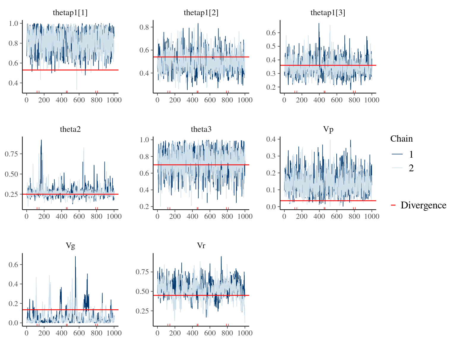
Figure 7.1: Parameters for Growth & Animal model: trace plots and expected values in red.
7.3 Genetic variance
We used the following growth model with a lognormal distribution to estimate individual growth potential and associated genotypic variation:
\[\begin{equation} DBH_{y=today,p,i} - DBH_{y=y0,p,i} \sim \\ \mathcal{logN} (log(\sum _{y=y_0} ^{y=today} \theta_{1,p,i}.exp(-\frac12.[\frac{log(\frac{DBH_{y,p,i}}{100.\theta_{2,p}})}{\theta_{3,p}}]^2)), \sigma_1) \\ \theta_{1,p,i} \sim \mathcal {logN}(log(\theta_{1,p}.a_{1,i}), \sigma_2) \\ \theta_{2,p} \sim \mathcal {logN}(log(\theta_2),\sigma_3) \\ \theta_{3,p} \sim \mathcal {logN}(log(\theta_3),\sigma_4) \\ a_{1,i} \sim \mathcal{MVlogN}(log(1), \sigma_5.K) \tag{7.3} \end{equation}\]
We fitted the equivalent model with the following priors:
\[\begin{equation} DBH_{y=today,p,i} - DBH_{y=y0,p,i} \sim \\ \mathcal{logN} (log(\sum _{y=y_0} ^{y=today} \hat{\theta_{1,p,i}}.exp(-\frac12.[\frac{log(\frac{DBH_{y,p,i}}{100.\hat{\theta_{2,p}}})}{\hat{\theta_{3,p}}}]^2)), \sigma_1) \\ \hat{\theta_{1,p,i}} = e^{log(\theta_{1,p}.\hat{a_{1,i}}) + \sigma_2.\epsilon_{1,i}} \\ \hat{\theta_{2,p}} = e^{log(\theta_2) + \sigma_3.\epsilon_{2,p}} \\ \hat{\theta_{3,p}} = e^{log(\theta_3) + \sigma_4.\epsilon_{3,p}} \\ \hat{a_{1,i}} = e^{\sigma_5.A.\epsilon_{4,i}} \\ \epsilon_{1,i} \sim \mathcal{N}(0,1) \\ \epsilon_{2,p} \sim \mathcal{N}(0,1) \\ \epsilon_{3,p} \sim \mathcal{N}(0,1) \\ \epsilon_{4,i} \sim \mathcal{N}(0,1) \\ ~ \\ (\theta_{1,p}, \theta_2, \theta_3) \sim \mathcal{logN}^3(log(1),1) \\ (\sigma_1, \sigma_2, \sigma_3, \sigma_4, \sigma_5) \sim \mathcal{N}^5_T(0,1) \\ ~ \\ V_P = Var(log(\mu_p)) \\ V_G=\sigma_5^2\\ V_R=\sigma_2^2 \tag{7.4} \end{equation}\]
| Parameter | Estimate | Standard error | \(\hat R\) | \(N_{eff}\) |
|---|---|---|---|---|
| thetap1[1] | 0.5423337 | 0.0699702 | 1.002517 | 1993 |
| thetap1[2] | 0.5596376 | 0.1084135 | 1.001838 | 2331 |
| thetap1[3] | 0.3485849 | 0.0301761 | 1.002514 | 1218 |
| theta2 | 0.2528277 | 0.0858377 | 1.005150 | 2249 |
| theta3 | 0.6963378 | 0.1038580 | 1.006909 | 1345 |
| sigma[1] | 0.1373708 | 0.0742090 | 1.356851 | 22 |
| sigma[2] | 0.5075622 | 0.1714122 | 1.107800 | 61 |
| sigma[3] | 0.2805989 | 0.2994495 | 1.000577 | 2627 |
| sigma[4] | 0.1377079 | 0.2346745 | 1.002896 | 2934 |
| sigma[5] | 0.4684783 | 0.1850532 | 1.068632 | 87 |
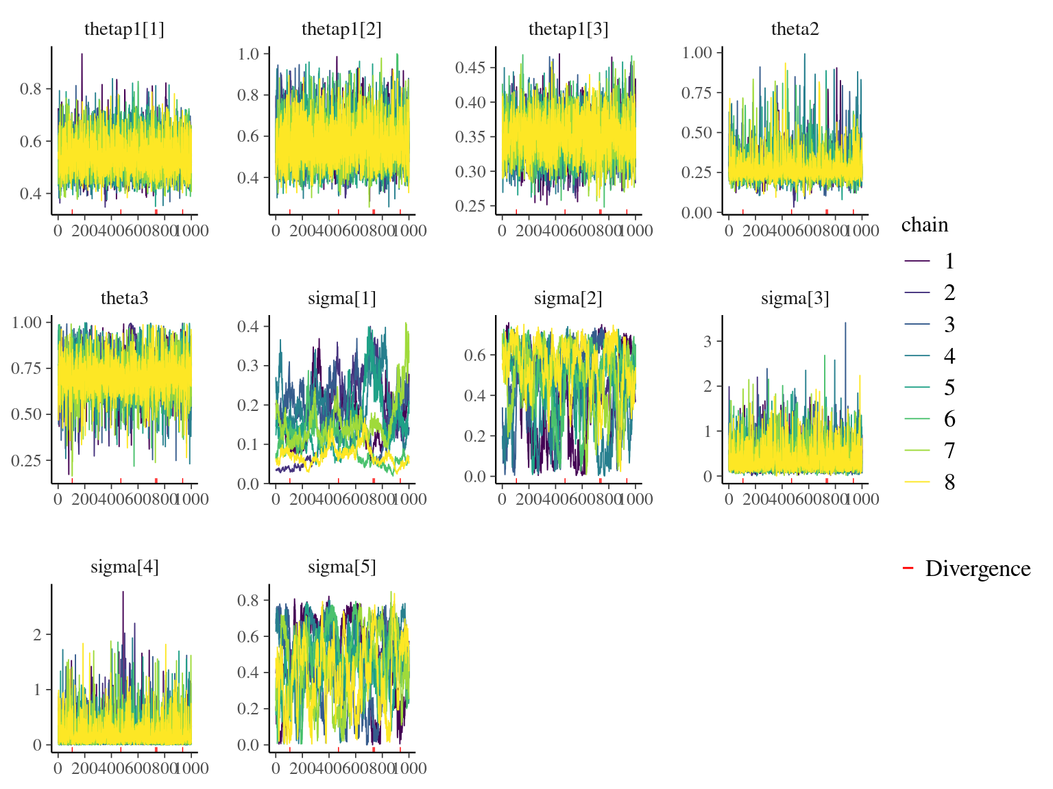
Figure 7.2: Trace plots of model parameters.
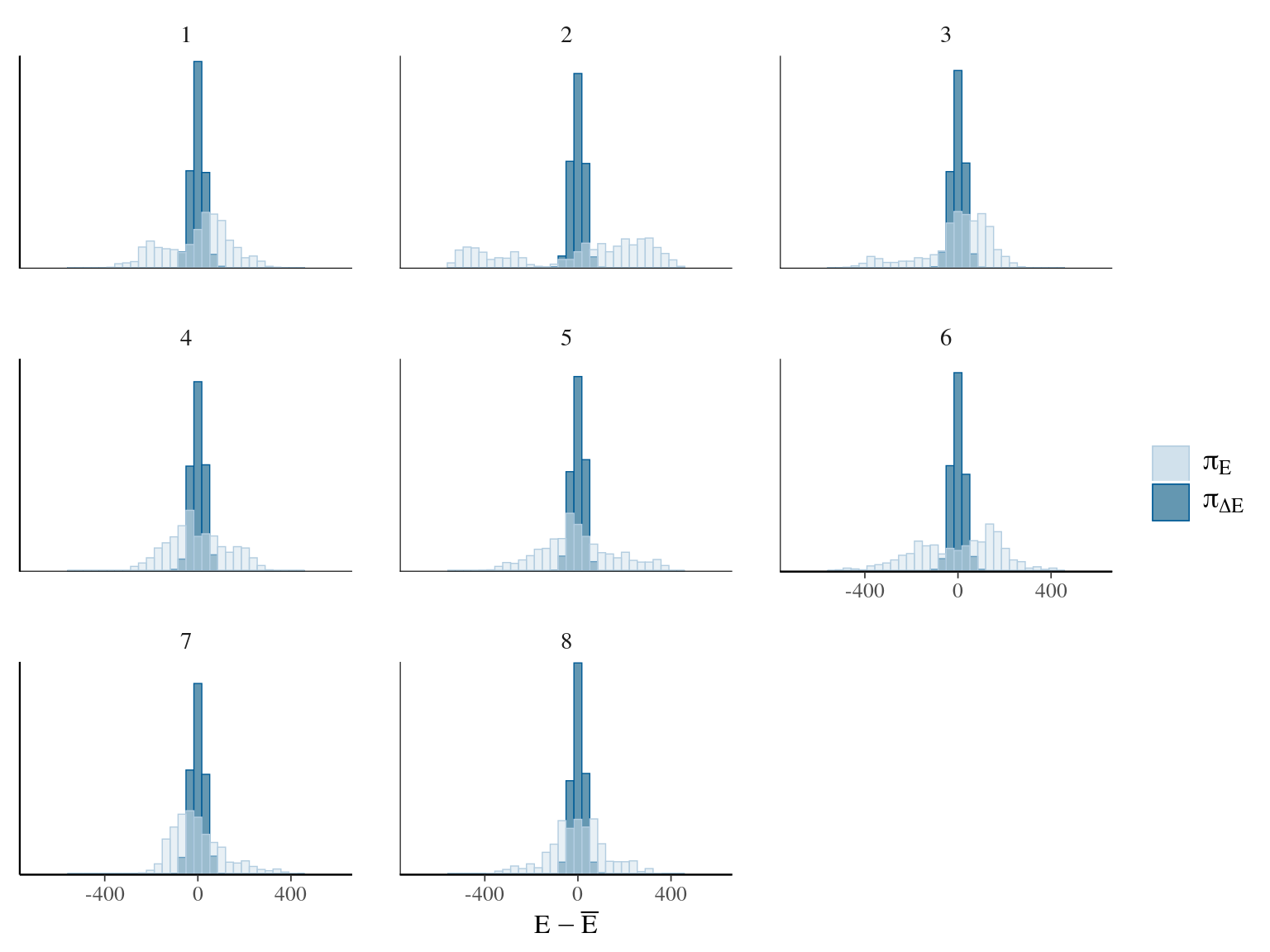
Figure 7.3: Energy of the model.
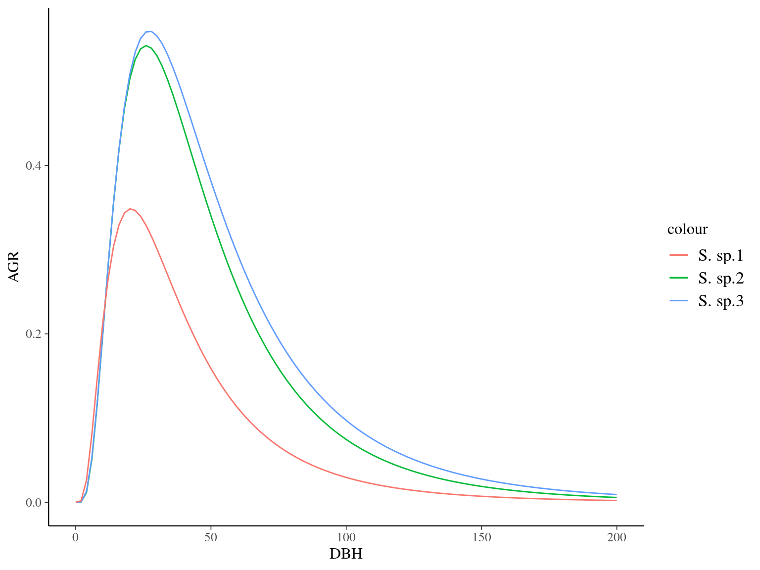
Figure 7.4: Species predicted growth curves.
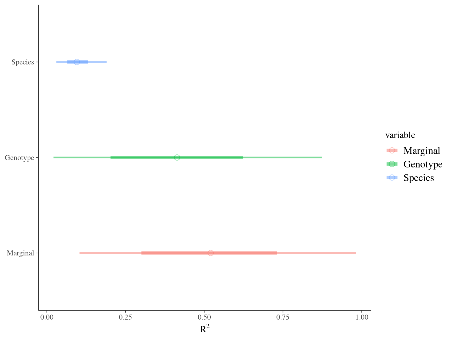
Figure 7.5: R2 for Gmax.
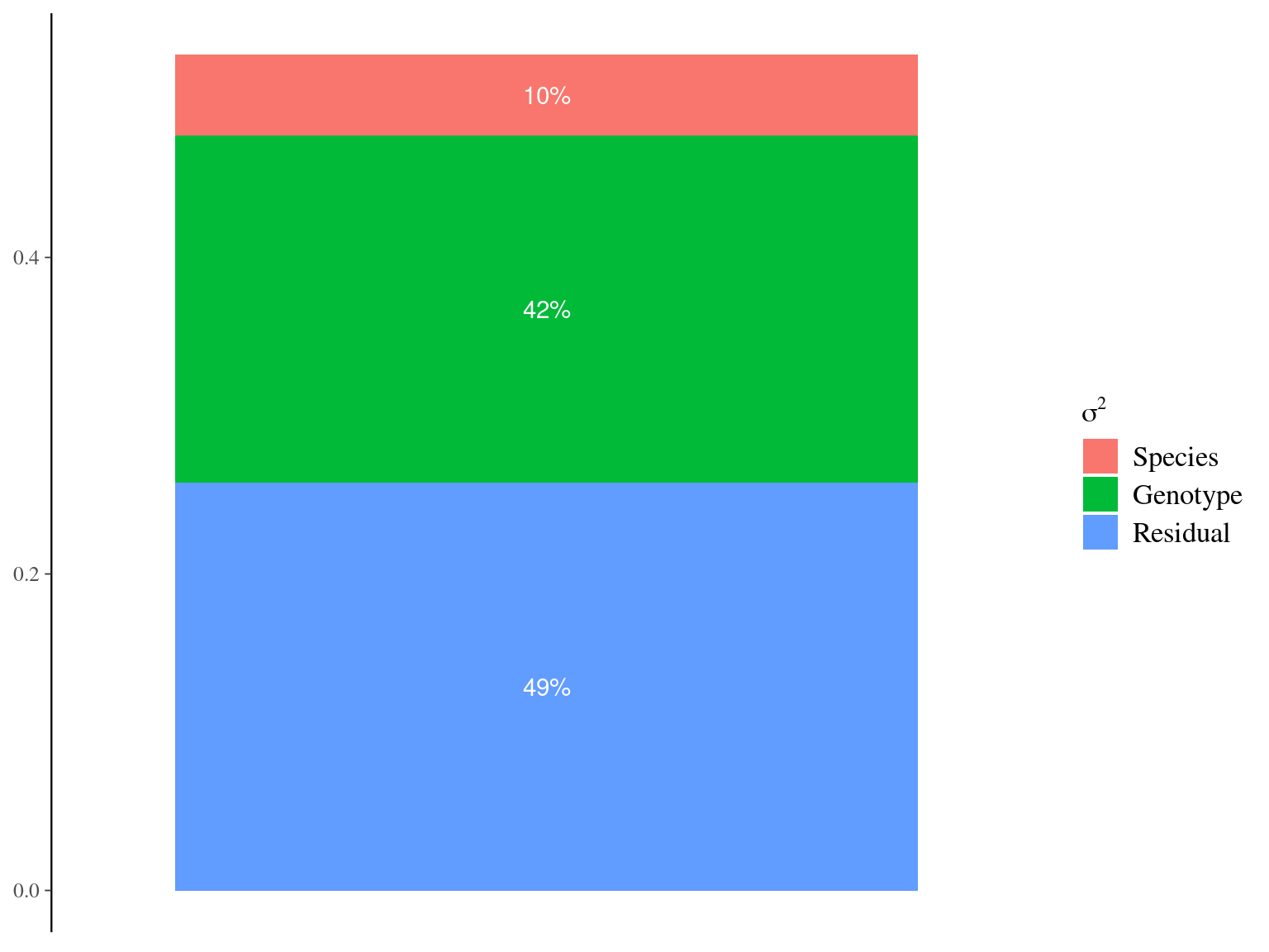
Figure 7.6: Genetic variance partitioning for Gmax.
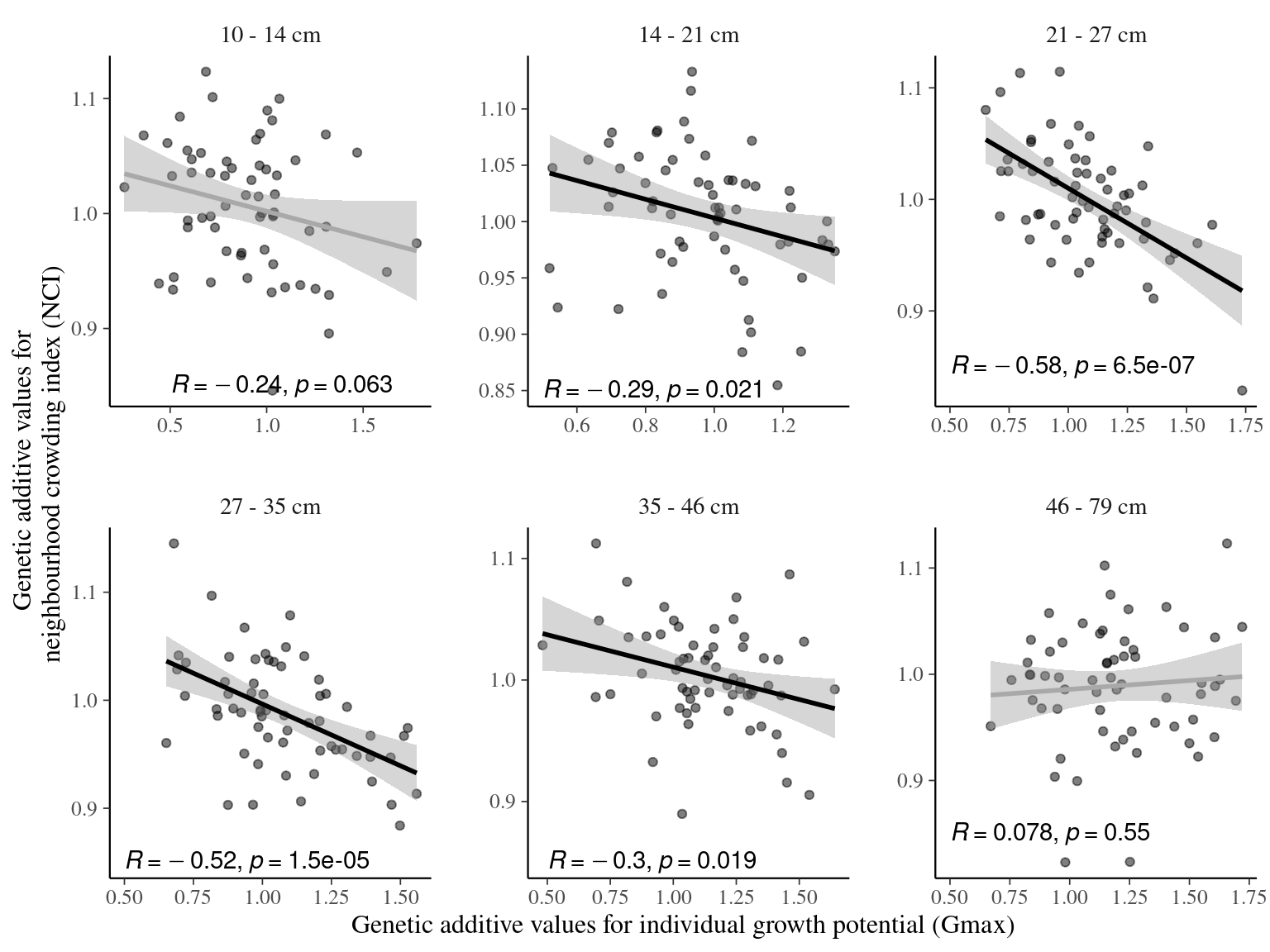
Figure 7.7: Relation between genotypic values for individual growth potential (Gmax) and neighbourhood crowding index (NCI), an indirect measurement of access to light, for different classes of diameters. Regression lines represent a linear model of form y ~ x. Annotations give for each diameter class the Pearson’s R correlation coefficient and the associated p-value.
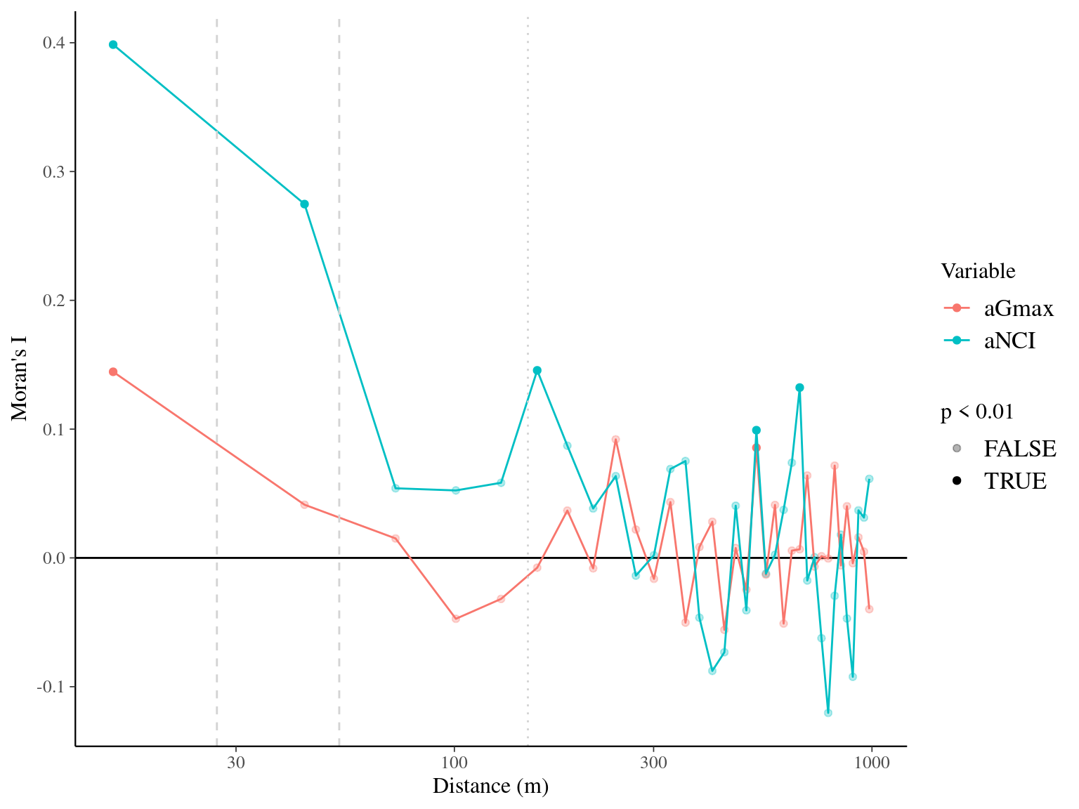
Figure 7.8: Spatial autocorrelogram (Moran’s I) of variables and associated genetic additive values (a).
7.4 Confounding phenotypic and environmental variation
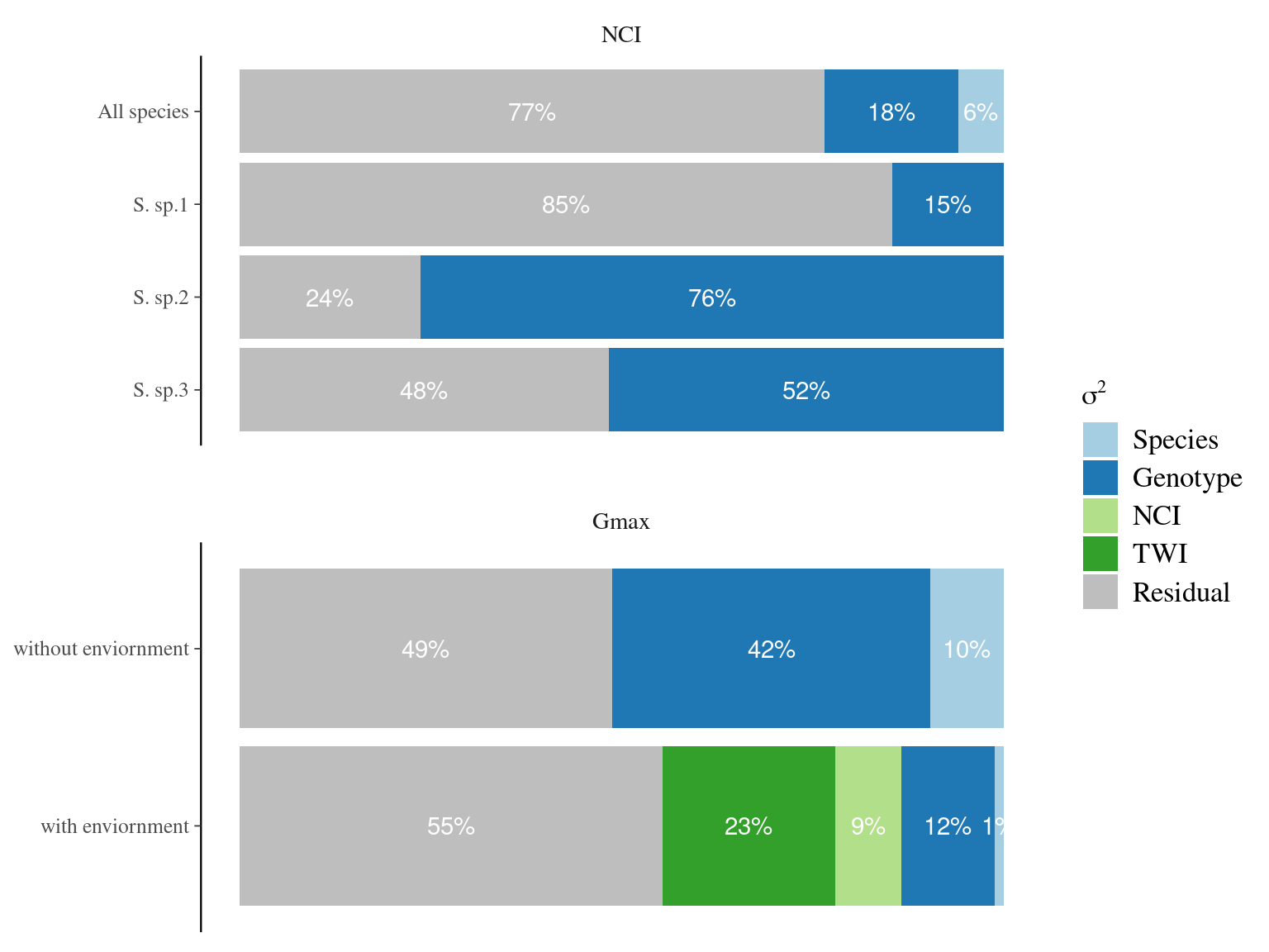
If the phenotypic variation is only plastic and confounded with the environmental variation, the genotypic variance associated to the phenotype while controlling for the environmental variation should be null (\(\sigma^2_{G|E}=0\)). Instead, we still observed a non null genotypic variation while controlling for the environmental variation (\(\frac{\sigma^2_{G|E}}{\sigma^2_P}=0.12\), Fig. 7.13).
We used the following growth model with a lognormal distribution to estimate individual growth potential and associated genotypic variation controlling for environmental variation (\(NCI\) and \(TWI\)) at the individual scale:
\[\begin{equation} DBH_{y=today,p,i} - DBH_{y=y0,p,i} \sim \\ \mathcal{logN} (log(\sum _{y=y_0} ^{y=today} \theta_{1,p,i}.exp(-\frac12.[\frac{log(\frac{DBH_{y,p,i}}{100.\theta_{2,p}})}{\theta_{3,p}}]^2)), \sigma_1) \\ \theta_{1,p,i} \sim \mathcal {logN}(log(\theta_{1,p}.a_{1,i}. \beta_1.TWI_i.\beta_2.NCI_i), \sigma_2) \\ \theta_{2,p} \sim \mathcal {logN}(log(\theta_2),\sigma_3) \\ \theta_{3,p} \sim \mathcal {logN}(log(\theta_3),\sigma_4) \\ a_{1,i} \sim \mathcal{MVlogN}(log(1), \sigma_5.K) \tag{7.5} \end{equation}\]
We fitted the equivalent model with following priors:
\[\begin{equation} DBH_{y=today,p,i} - DBH_{y=y0,p,i} \sim \\ \mathcal{logN} (log(\sum _{y=y_0} ^{y=today} \hat{\theta_{1,p,i}}.exp(-\frac12.[\frac{log(\frac{DBH_{y,p,i}}{100.\hat{\theta_{2,p}}})}{\hat{\theta_{3,p}}}]^2)), \sigma_1) \\ \hat{\theta_{1,p,i}} = e^{log(\theta_{1,p}.\hat{a_{1,i}}. \beta_1.TWI_i.\beta_2.NCI_i) + \sigma_2.\epsilon_{1,i}} \\ \hat{\theta_{2,p}} = e^{log(\theta_2) + \sigma_3.\epsilon_{2,p}} \\ \hat{\theta_{3,p}} = e^{log(\theta_3) + \sigma_4.\epsilon_{3,p}} \\ \hat{a_{1,i}} = e^{\sigma_5.A.\epsilon_{4,i}} \\ \epsilon_{1,i} \sim \mathcal{N}(0,1) \\ \epsilon_{2,p} \sim \mathcal{N}(0,1) \\ \epsilon_{3,p} \sim \mathcal{N}(0,1) \\ \epsilon_{4,i} \sim \mathcal{N}(0,1) \\ ~ \\ (\theta_{1,p}, \theta_2, \theta_3) \sim \mathcal{logN}^3(log(1),1) \\ (\sigma_1, \sigma_2, \sigma_3, \sigma_4, \sigma_5) \sim \mathcal{N}^5_T(0,1) \\ ~ \\ V_P = Var(log(\mu_p)) \\ V_G=\sigma_5^2\\ V_{TWI} = Var(log(\beta_1.TWI_i)) \\ V_{NCI} = Var(log(\beta_2.NCI_i)) \\ V_R=\sigma_2^2 \tag{7.6} \end{equation}\]
| Parameter | Estimate | Standard error | \(\hat R\) | \(N_{eff}\) |
|---|---|---|---|---|
| thetap1[1] | 0.6819703 | 0.1750196 | 1.0017710 | 3771 |
| thetap1[2] | 0.4693647 | 0.1630881 | 1.0003561 | 3238 |
| thetap1[3] | 0.7133448 | 0.1741461 | 1.0009126 | 3999 |
| beta[1] | 1.0338461 | 0.4773498 | 1.0009493 | 5751 |
| beta[2] | 1.0231845 | 0.4821474 | 0.9998852 | 6093 |
| theta2 | 0.2212118 | 0.0872344 | 1.0031382 | 1564 |
| theta3 | 0.6542952 | 0.1080025 | 1.0011451 | 2755 |
| sigma[1] | 0.1302832 | 0.0953805 | 1.3708842 | 22 |
| sigma[2] | 0.8841277 | 0.1185958 | 1.1145255 | 81 |
| sigma[3] | 0.3078621 | 0.3262250 | 1.0020929 | 2855 |
| sigma[4] | 0.1441136 | 0.2493211 | 1.0005756 | 4162 |
| sigma[5] | 0.4157660 | 0.2270843 | 1.1430011 | 55 |
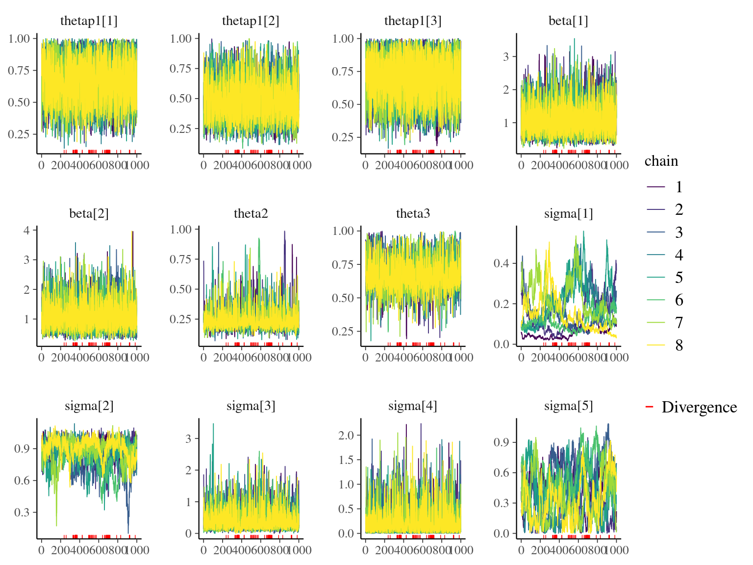
Figure 7.9: Traceplot of model parameters.
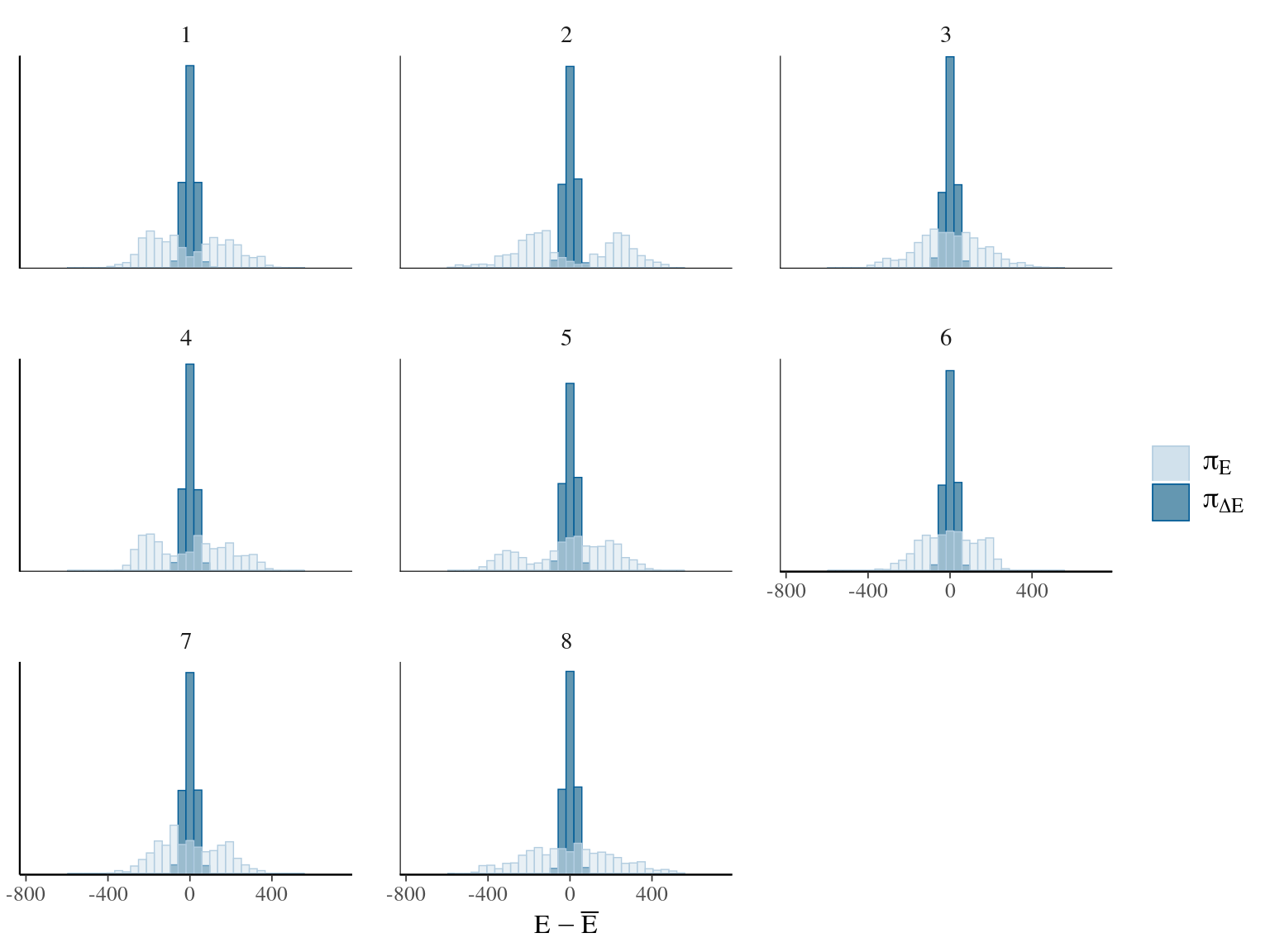
Figure 7.10: Energy of the model.
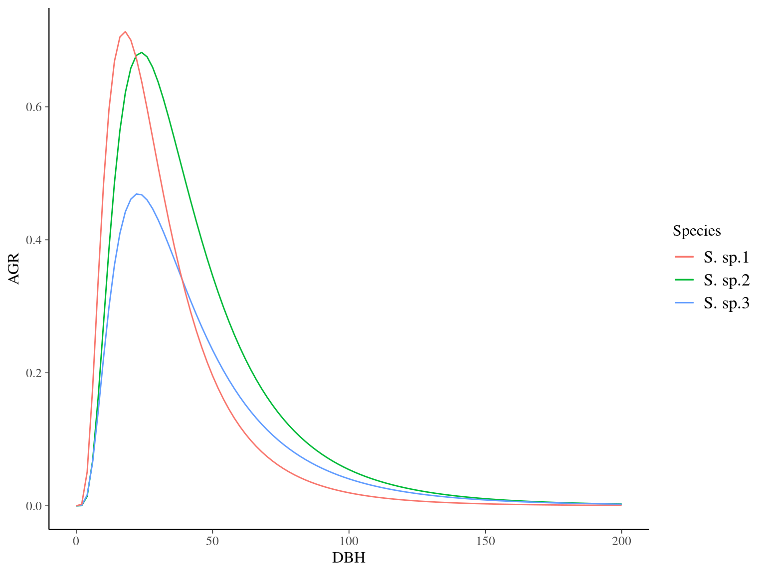
Figure 7.11: Species predicted growth curve.
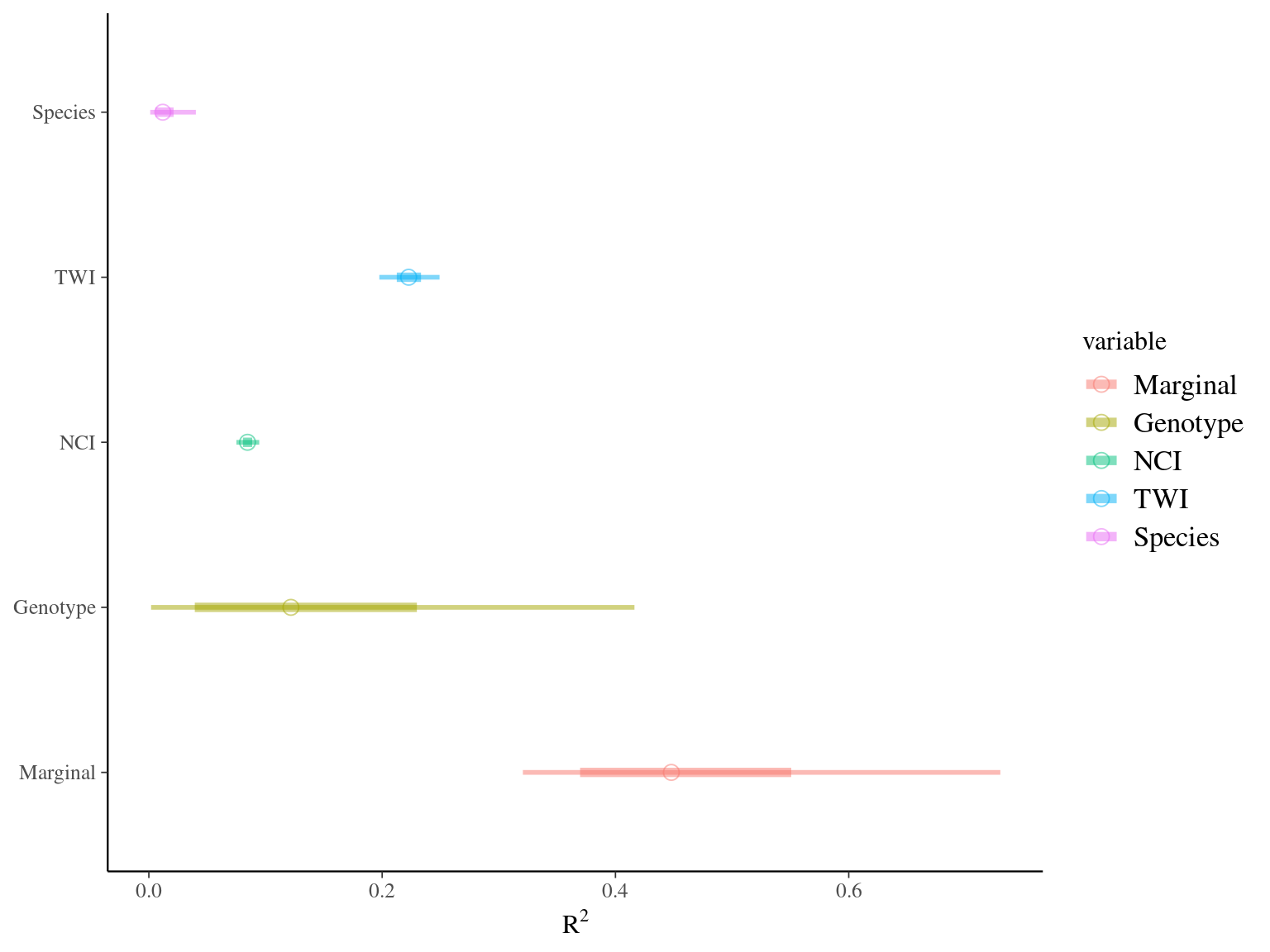
Figure 7.12: R2 for Gmax.
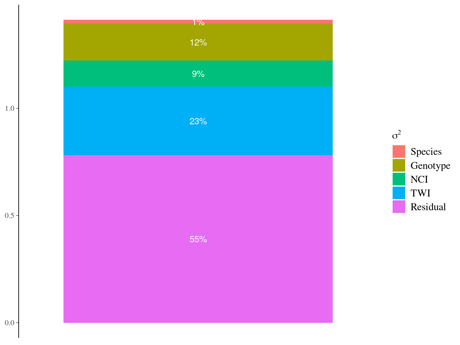
Figure 7.13: Variance partitioning for individual maximum growth potential (Gmax). Variation of individual maximum growth potential has been partitioned into among-species (red), among-genotype (brown), along forest gap dynamics (NCI, green), along topography (TWI, blue), and residual (pink) variations.
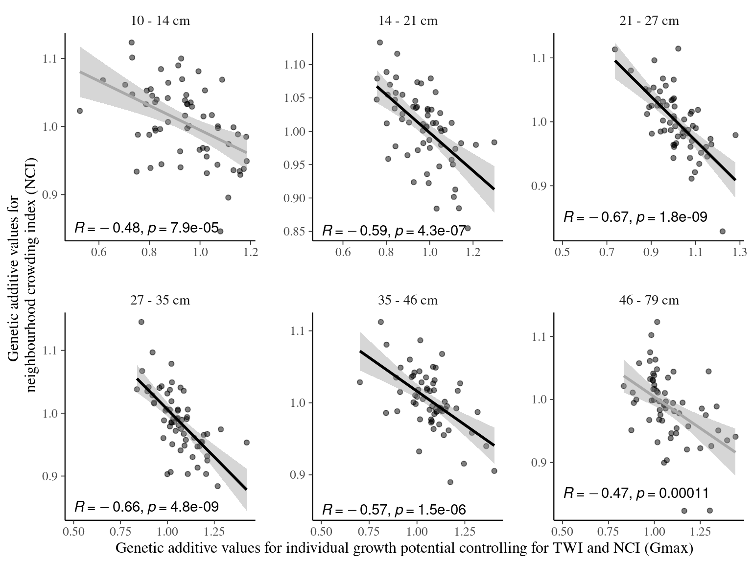
Figure 7.14: Relation between genotypic values for individual growth potential controlling for TWI and NCI (Gmax) and neighbourhood crowding index (NCI), an indirect measurement of access to light, for different classes of diameters. Regression lines represent a linear model of form y ~ x. Annotations give for each diameter class the Pearson’s R correlation coefficient and the associated p-value.
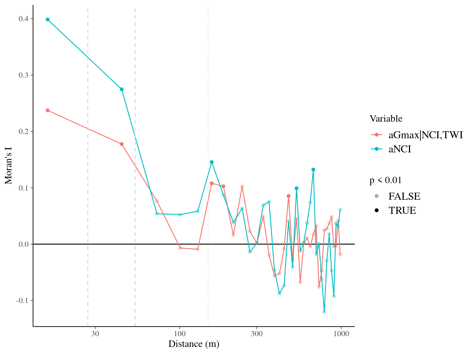
Figure 7.15: Spatial autocorrelogram (Moran’s I) of variables and associated genetic multiplicative values.
7.5 Manuscript figure
References
Carpenter, B., Gelman, A., Hoffman, M.D., Lee, D., Goodrich, B., Betancourt, M., Brubaker, M., Guo, J., Li, P. & Riddell, A. (2017). Stan : A Probabilistic Programming Language. Journal of Statistical Software, 76. Retrieved from http://www.jstatsoft.org/v76/i01/
Gompertz, B. (1825). On the nature of the function expressive of the law of humanmortality, and on a newmode of determining the value of life contingencies. Philosophical Transactions of the Royal Society of London, 115, 513–583. Retrieved from https://www.tandfonline.com/doi/full/10.1080/14786445908642737
Hérault, B., Bachelot, B., Poorter, L., Rossi, V., Bongers, F., Chave, J., Paine, C.E.T., Wagner, F. & Baraloto, C. (2011). Functional traits shape ontogenetic growth trajectories of rain forest tree species. Journal of Ecology, 99, 1431–1440.
Hoffman, M.D. & Gelman, A. (2014). The no-U-turn sampler: Adaptively setting path lengths in Hamiltonian Monte Carlo. Journal of Machine Learning Research, 15, 1593–1623. Retrieved from http://arxiv.org/abs/1111.4246
Nakagawa, S. & Schielzeth, H. (2013). A general and simple method for obtaining R2 from generalized linear mixed-effects models. Methods in Ecology and Evolution, 4, 133–142.