2 Material and Methods
2.1 Sensitivity analysis
Maréchaux & Chave already assessed TROLL model sensitivity to several parameters (\(k\) see (A.2), \(\phi\) see (A.25), \(g1\) see (A.6), \(f_{wood}\) see (A.14), \(f_{canopy}\) see (A.16) and \(m\) see (A.21)) which they assumed having a key role in model functioning. On the other hand, we decided to use TROLL to study resistance and resilience of ecosystem face to disturbance, highlighting the role of biodiversity. Consequently we particulrarly needed to assess the importance of functional traits to further better control and evaluate functional diversities. We also needed to assess the sensitivity of TROLL model to the seed rain constant (\(n_{ext}\), see (A.24)) because we assumed it was one of the main factors of tree recruitments after disturbance within simulations.
TROLL model currenty uses leaf mass per area (\(LMA\) in \(g.m^{-2}\)), leaf nitrogen content per dry mass (\(N_m\) in \(mg.g^{-1}\)), leaf phosphorus content per dry mass (\(P_m\) in \(mg.g^{-1}\)), wood specific gravity (\(wsg\) in \(g.cm^{-3}\)), diameter at breasth height threshold (\(dbh_{thresh}\) in \(m\)), asymptotic height (\(h_{lim}\) in \(m\)), and parameter of the tree-height-dbh allometry (\(a_h\) in \(m\)). To assess the sensitivity of TROLL model to species functionnal traits, we performed a sensitivity analysis by fixing species trait values to their mean. Each trait was tested independently. We reduce to a common mean traits with a Pearson’s correlation value \(r \geq 0.8\) (\(h_{max}\) and \(a_h\) with a correlation of \(r=0.98\)). To assess the sensitivity of TROLL model to seed rain, we performed a sensitivity analysis by fixing simulations seed rain constant to 2, 20, 200 and 2000 seeds per hectare.
Simulations were conducted on Intel Xeon(R) with 32 CPUs of 2.00GHz and 188.9 GB of memory. We assumed maturity of the forest after 500 years of regeneration Maréchaux & Chave and computed simulation 100 years after a disturbance event with 40% loss of basal area. Due to computer limitations we did not run replicates (besides it should be necessary to reduce simulation stochasticity). To assess ecosystem outputs sensitivity to studied parameters, we compared it to 100 replicates of control simulations with all parameters set to default values. Ecosystem outputs outside of the range of the control replicates values are significantly influenced by the studied parameter.
2.2 Design of experiment
In order to assess the role of biodiversity in ecosystem answer to both disturbance and sylviculture, we needed to create a space of experiments encompassing both variation of disturbance, biodiversity and time. Disturbance was represented by percentage of basal area loss (0%, 25%, 50% and 75%), or as a selective logging simulation using default parameters. Biodiversity was integrated with two of its components: taxonomic and functional diversities. We used species richness \(SR\) to represents taxonomic diversity (5, 25, and 125 species). Functional diversity can be related to numerous components, and Perrone et al. (2017) argued for 5: richness, divergence, regularity, overlap and mean. Because mature forest were created from a bare soil with TROLL simulations, we could not control a priori divergence, regularity and overlap but only assess them after running the simulations, i.e. before applying the diturbance. Consequently, we focused on functional richness with convex hull volume \(CHV\) and functional mean with community weighted mean \(CWM\). For each level of species richness \(SR\), we selected 20 communities with growing convex hull volume \(CHV\) but with a community weighted means close to the regional species pool community weighted means. Effectivelly, we did not wanted drastic change in community means that could have more effect than functional richness itself. This design of experiments resulted in 60 communities (\(5~SR*20~CHV\)) and 240 simulations (\(60 ~communities*4~levels~of~disturbance\)) over 600 years (maturity being assumed after 500 years of regeneration (Maréchaux & Chave)). Functional diversities of mature forests were assessed with Villéger et al. (2008) indices (FRIC, FEve, FDiv, and FDis). Figure 2.1 presents the design of experiment for communities biodiversity after the mature forest were simulated, and thus before disturbance. We obtained a broad range of both functionl dispersion \(FDis\) and aboveground biomass \(AGB\) for simulated forest ecosystems before disturbance.
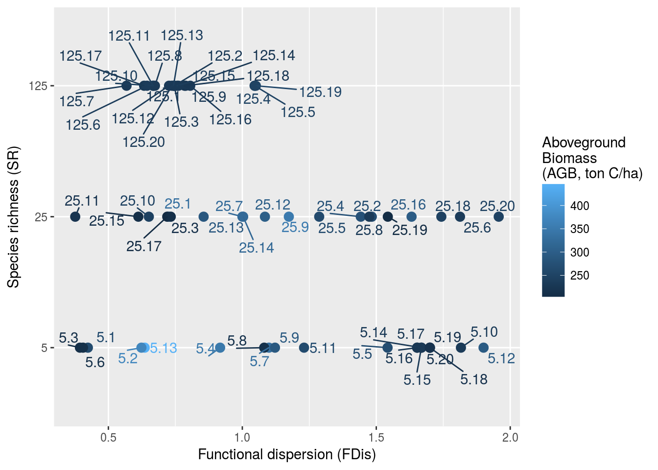
Figure 2.1: Experimental design before disturbance. Communities are implemented along a gradient of species richness (SR) and functional dispersion (FDis) resulting in a broad range of aboveground biomass (AGB). FDis was caluclated based on 4 functional traits (leaf mass per area, wood specific gravity, maximum diameter, and maximum height).
2.3 Ecosystem response analysis
2.3.1 Ecosystem functions
Tropical forest ecosystems provides numerous ecosystem services linked to several ecosystem functions. We decided to describe simulated tropical forests in two major functions: forest structure and forest functionning. Forest structure was represented by aboveground biomass (\(AGB\) in \(ton~C.ha^{-1}\)), basal area (\(BA\) in \(m^2.ha^{-1}\)), total number of stem (\(N\)), number of stem above \(10~cm\) diameter (\(N10\)), and number of stem above \(30~cm\) diameter (\(N30\)). Forest functionning was represented by growth primary productivity (\(GPP\) in \(MgC.ha^{-1}\)), net primary productivity (\(NPP\) in \(MgC.ha^{-1}\)), tree autotrophic respiration in day (\(Rday\) in \(MgC.ha^{-1}\)) and tree autotrophic respiration in night (\(Rnight\) in \(MgC.ha^{-1}\)).
The resilience of metrics values post disturbance were assessed through Henry & Emmanuel Ramirez-Marquez (2012) formula:
\[\begin{equation} R\left(t\right)=\frac{Recovery\left(t\right)}{Loss\left(t_d\right)} \approx \frac{X_T(t)}{X_C(t)} \tag{2.1} \end{equation}\]The resilience of the system \(R(t)\) at the time \(t\) is described by the ratio of recovery \(Recovery(t)\) at time \(t\) to loss suffered \(Loss(t_d)\) at disturbance time \(t_d\). But in our peculiar case of tropical forest ecosystems, the equilibrium used to calculate \(Loss(t_d)\) can not be reduced to a specific time if the equilibrium is dynamic. Consequently, to encompass undisturbed ecosystem variations throught time, we simulated an undisturbed control ecosystem \(C\). And the resilience of the system \(R(t)\) at the time \(t\) was defined as the ratio of the ecosystem metric values in the disturbed simulation \(X_T(t)\) over the ecosystem metric values from the control \(X_C(t)\) . Thus, the value of resilience \(R(t)\) is normalized for all simulations and metrics. \(R(t)\) will be equal to \(R_{eq} = 1\) when reaching the equilibrium value. Consequently we can calculate an euclidean distance to equilibrium \(d_{eq}(t)\) as \(d_{eq}(t) = \sqrt{(R_{eq} - R(t))^2}\). Ecosystem euclidean distance to equilibrium was calculated in a multi-dimensional space for the two functions described above: forest strcuture (AGB, BA, N, N10, and N30) and forest functionning (GPP, NPP, Rday, and Rnight). We then used integrated eulcidean distance to equilibrium over time to assess simulations resilience.
2.3.2 Biodiversity effect
Biodiversity is not only a facet of the experimental design and an ecosystem output through forest diversity, but also interact on ecosystem functioning and consequently on its answer to disturbance. Biodiversity ecosystem functioning relation can be split in complementarity and selection effect with Loreau & Hector (2001b) partitioning:
\[\begin{equation} \begin{array}{c} NE = X_O - X_E = CE + SE \\ CE = N* \overline{\Delta RX} \overline{M}\\ SE = N*cov(\Delta RX,M) \end{array} \tag{2.2} \end{equation}\]Biodiversity net effect \(NE\) is based on the difference between ecosystem variable \(X\) observed value \(X_O\) within the community mixture of species and its expected value \(X_E\) if species performance were equal to their performance in monocultures. This effect can be partitioned between complementarity effect \(CE\), representing niche partitionning, positive interactions, and resource supply, and selectvie effect \(SE\) due to dominant species pool driving the ecosystem. \(N\) represents the total number of species, and \(M\) the vector of monocultures performance. Both metrics depend on the variation of relative ecosystem variable \(\Delta RX\):
\[\begin{equation} \Delta RX_{sp} = \frac{X_{sp}(mixture)}{X_{sp}(monoculture)} - P_{sp} \tag{2.3} \end{equation}\]\(X_{sp}\) is the ecosystem variable value for one species either in mixture \(X_{sp}(mixture)\) or in monoculture \(X_{sp}(monoculture)\). \(P_{sp}\) is the proportion of the species in the mixture represented by species relative abundance. Consequently, \(CE\) averages diversity effects of all species presents in the mixture (both negatives and positives). Whereas \(SE\) become positive when dominant species outperform themselves in mixture than in monoculture, and negative when less dominant species outperform themselves in mixture than in monoculture (Tobner et al. 2016). But similarly to resilience measurement, biodiversity net effect \(NE\) is a dynamic equilibrium and vary over time without disturbance. So in order to correctly assess selection and complementarity effect in answer to disturbance, we normalized it by undisturbed control ecosystem net effect \(NE_C\) to measure treatments net effect resilience \(R(NE_T)\):
\[\begin{equation} R(NE_T) = \frac{NE_T}{NE_C} = \frac{SE_T}{NE_C} + \frac{CE_T}{NE_C} \tag{2.4} \end{equation}\]Resilience trajectories of ecosystem variable after disturbance were partitioned between complementarity effect \(CE\) and selection effect \(SE\). In order to do that, the design of experiment was repeated for each species indivdually representing 652 simulations of monoculture.
References
Perrone, R., Munoz, F., Borgy, B., Reboud, X. & Gaba, S. (2017). How to design trait-based analyses of community assembly mechanisms: insights and guidelines from a literature review. Journal of PPEES Sources, 25, 29–44.
Villéger, S., Mason, N.W.H. & Mouillot, D. (2008). New multidimensional functional diversity indices for a multifaceted framework in functional ecology. Ecology, 89, 2290–2301.
Henry, D. & Emmanuel Ramirez-Marquez, J. (2012). Generic metrics and quantitative approaches for system resilience as a function of time. Reliability Engineering and System Safety, 99, 114–122.
Loreau, M. & Hector, a. (2001b). Partitioning selection and complementarity in biodiversity experiments. Nature, 412, 72–6.
Tobner, C.M., Paquette, A., Gravel, D., Reich, P.B., Williams, L.J. & Messier, C. (2016). Functional identity is the main driver of diversity effects in young tree communities (F. He, Ed.). 19, 638–647.