1 Model description

1.1 Overview

TROLL model each tree indivdually in a located environment. Thus TROLL model, alongside with SORTIE (Pacala et al. 1996; Uriarte et al. 2009) and FORMIND (Köhler & Huth 1998; Fischer et al. 2016), can be defined as an individual-based and spatially explicit forest growth model. TROLL simulates the life cycle of individual trees from recruitment, with a diameter at breast height (dbh) above 1 cm, to death with growth and seed production. Trees are growing in a spatialized light environment explicitly computed witin voxels of 1 \(m^3\). Each tree is consistently defined by its age, diameter at brest height (dbh), height (h), crown radius (CR), crown depth (CD) and leaf area (LA) (see figure 1.1). Tree geometry is calculated with allometric equations but leaf area vary dynamically within each crown following carbon allocations. Voxels resolution of 1 \(m^3\) allow the establishment of maximum one tree by 1x1 m pixels. Each tree is flagged with a species label inherited from the parent tree through the seedling recruitment. A species label is associated to a number of species specific parameters (see table 1.1) related to functional trait values which can be sampled on the field.

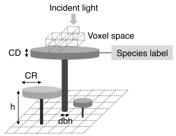
Figure 1.1: Individuals tree inside TROLL explicit spatial grid from Maréchaux & Chave. Tree geometry (crown radius CR, crown depth CD, height h, diameter at breast height dbh) is updated at each timestep following allometric relationship with assimilated carbon allocated to growth. Each tree is flagged with a species label linking to its species-specific attributes. Light is computed explicitly at each timestep for each voxel.

Carbon assimilation is computed over half-hourly period of a representative day. Then allocation is computed to simulate tree growth from an explicit carbone balance (in contrast to previous models). Finally environment is updated at each timestep set to one month. Seedlings are not simulated explicitly but as a pool. In addition belowground processes, herbaceous plants, epiphytes and lianas are not simulated inside TROLL. The source code is written in C++ and available upon request. All modules of TROLL models are further detailed in Appendix 1: TROLL model.

Table 1.1: Species-specific parameters used in TROLL from Maréchaux & Chave. Data originates from the BRIDGE (Baraloto et al. 2010) and TRY (Kattge et al. 2011) datasets.

Abbreviation	Description	Units
\(LMA\)	leaf mass per area	\(g.m^{-2}\)
\(N_m\)	leaf nitrogen content per dry mass	\(mg.g^{-1}\)
\(P_m\)	leaf phosphorous content per dry mass	\(mg.g^{-1}\)
\(wsg\)	wood specific gravity	\(g.cm^{-3}\)
\(dbh_{thresh}\)	diameter at breasth height threshold	\(m\)
\(h_{lim}\)	asymptotic height	\(m\)
\(a_h\)	parameter of the tree-height-dbh allometry	\(m\)

Previous implementation of TROLL model used Reich et al. (1991) allometry to infer leaf lifespan \(LL\) from species leaf mass per area \(LMA\) (Maréchaux & Chave, see Appendix 1: TROLL model). But the use of the allometrie from Reich et al. (1991) with current implementation of the TROLL model resulted in an underestimation of leaf lifespan for low LMA species. Consequently in the following paragraph we suggest a new allometry.

Selective logging is defined as the targeted harvesting of timber from species of interest. Consequently, tropical sylviculture can be assimilated to a disturbance. The main difference between a disturbance and selective logging is the targetting of both species and individuals of interest. So we decided to first asses unselective disturbance effect on tropical forest ecosystem to subsequently better understand selective logging effect. First, we implemented a disturbance module inside TROLL model to simulate unselective disturbance. Secondly, we implemented a sylviculture module inside TROLL model to simulate selective logging in regards to french Guiana practices.

1.2 Leaf lifespan

The underestimation of leaf lifespan for low LMA species with the allometry from Reich et al. (1991) resulted in indivduals unealistic early death from carbon starvation. We gathered data from TRY(Kattge et al. 2011), DRYAD (Chave et al. 2009) and GLOPNET (Wright et al. 2004) datasets. We used an out of the bag method applied on a random forest to select variables with highest importance to explain leaf lifespan. We thus selected leaf mass per area \(LMA\), leaf nitrogen content \(N\) and wood specific gravity \(wsg\). We then used a bayesian approach to test different models with growing level of complexity. The model with the best tradeoff between complexity (number of parameters), convergence, likelihood, and prediction quality (root mean square error of prediction RMSEP) was kept. We selected following model with a maximum likelihood of 13.6 and a RMSEP of 12 months:

\[\begin{equation} LL_{d} \sim log\mathcal{N}({\beta_1}_d*LMA - {\beta_2}_d*N*\beta_3*wsg, \sigma) \tag{1.1} \end{equation}\]

Leaf lifespan \(LL\) follows a lognormal law with location infered from leaf lifespan \(LMA\), nitrogen content \(N\) and wood specific gravity \(wsg\) and a scale \(\sigma\). Each \({\beta_i}_d\) is following a normal law located on \(\beta_i\) with a scale of \(\sigma_i\). All \(\beta_i\), \(\sigma_i\), and \(\sigma\) are assumed without presemption following a gamma law. \(d\) represents the dataset random effects and encompass environmental and protocol variations (see Appendix 2: Leaf lifespan model for more details).

1.3 Disturbance

Disturbance module was designed in the simplest way in order to relate the ecosystem answer to volume loss without any individuals nor species targetting. For a given iteration \(disturb_{iter}\), individuals are picked randomly with a uniform law on the number of trees. Selected individuals are then removed without trigerring a treefall to avoid any side effect. The operation is repeated untill the disturbance result in a defined lost basal area (\(disturb_{intensity}\) in % of BA).

1.4 Sylviculture

In french guiana context, sylviculture can be narrow to selective logging, which can be split in two steps: selection and harvesting. Selection encompass choice of the havrestable area, harvestable tree designation by the forest office, harvested tree selection by the harvester, and removal off tree probbed as rotten by the lumber. Harvesting encompass tree felling, tracks opening, and long term damages (simplified in gap damages in current TROLL implementation).

1.4.1 Designation and selection

One major limit of current implementation of TROLL model is that it assumes a flat environment. Consequently the whole simulated area inside TROLL is considered has an harvestable zone. With all commercial species minimum and maximum harvestable diameter, TROLL calculates the total harvestable volume \({V_h}_{tot}\). If the total harvestable volume \({V_h}_{tot}\) exceed \(30~m^3.hectare^{-1}\), commercial species minimum harvestable diameter \(dbh_{min}\) is increased untill \({V_h}_{tot}\) is inferior to that upper limit.

In french guiana, tree harvesters are focusing on few species with easier marketable wood, resulting in a tree harvest around \(20~m^3.ha^{-1}\) (Laurent Descroix, ONF, personnal communication). TROLL ranks each commercial species on its economic value, and randomly remove individuals from lowest rank species untill it reaches total harvested volume \({V_{hd}}_{tot}\) (\({V_{hd}}_{tot}\) was set to \(25~m^3.hectare^{-1}\) in subsequent simulations).

1.4.2 Rotten trees

20 to 30 % of designated trees are considered as rotten once probed by the lumberman, and thus not harvested. Rotten trees are not random and depends both on tree species and diameter. We gathered data from the forest office (ONF, Laurent Descroix, personnal communication) inventories precising if tree were probbed as rotten and their corresponding species and diameter. In addition, tree plots and sawed volume was informed. We then used a bayesian approach to model the link between tree species and diameter and their risk to be probbed as rotten by the lumberman. We test different models with growing level of complexity and kept the model with the best tradeoff between complexity (number of parameters), convergence, likelihood, and prediction quality (root mean square error of prediction RMSEP):

\[\begin{equation} \begin{array}{c} probbed~rotten \sim \mathcal{B}(P(probbed~rotten)) \\ P(probbed~rotten) = logit^{-1}(\beta_0 + \beta_1*dbh) = \frac{e^{\beta_0 + \beta_1*dbh}}{1 + e^{\beta_0 + \beta_1*dbh}} \end{array} \tag{1.2} \end{equation}\]

Tree \(probbed~rotten\) follows a \(Bernoulli\) law of probability \(P(probbed~rotten)\). The odds for a tree to be probbed as rotten are calculated with the sum of a base odd to be rotten \(\beta_0\) and a diameter dependent odd calculated with \(\beta_1\). The probability for a tree to be probbed as rotten \(P(probbed~rotten)\) is finally calculated by taking the inverse logit \(logit^{-1}\) of the odd (see Appendix 3: Rotten tree model for more details).

1.4.3 Harvesting

Due to crown aspects, treefall from logs are often random (whereas difficult to manage, treefall can still be oriented, Laurent Descroix, ONF, personnal communication). Consequently, TROLL consider treefall from log as random like current natural treefall implementation inside TROLL (see code [Appendix 1]).

Tree harvesting roads are split in three classes: truck roads, main tractor track, and secondary track. Because TROLL assumes a flat environment, the main track is opened starting from the midle of one side of the simulated forest and untill it reaches the center with a width of 6 meters. In most cases, secondary tracks are opened once trees have been designated and the geolocation taken at a maximum distance of 30 meters from designated trees (Laurent Descroix, ONF, personnal communication). To simulate secondary tracks, TROLL uses a loads map, measuring every trees at a distance of 30 meters for each pixel, and a track proximity maps of the closest existing track. Next, the model select the pixel with the highest load and closest track, find the closest existing track and join it by removing tree in the way with a width of 5 meters. The operations are repeated untill no felt trees are left.

1.4.4 Gap damages

Most of models account long term damages due to selective logging with a 10 years increased mortality (Huth et al. 2004; Köhler & Huth 2004; Rüger et al. 2008). We decided to model explicitly long term logging damages because of their localised nature through a gap damages model. We gathered data from Paracou dataset (Guehl et al. 2004) in cenususes between 1988 and 1992 on Paracou harvested plots. Individuals were categorized between alive, dead, or recruited during the period. We measured each individual distance to the closest gap. We then used a bayesian approach to test the link between tree death in the four years following the log event and distance to the closest gap. We adapted the model from Herault et al. (2010) based on a disturbance index into:

\[\begin{equation} \begin{array}{c} Death \sim \mathcal{B}(P(Death)) \\ P(Death) = logit^{-1}(\theta + \beta*e^{\alpha*d_{gaps}}) = \frac{e^{\theta + \beta*e^{\alpha*d_{gaps}}}}{1 + e^{\theta + \beta*e^{\alpha*d_{gaps}}}} \end{array} \tag{1.3} \end{equation}\]

\(Death\) of a tree follows a \(\mathcal{B}ernoulli\) law of probability \(P(Death)\). The odds for a tree to die are calculated with the sum of the natural tree death odd \(\theta\) and a perturbation index \(\beta*e^{\alpha*d_{gaps}}\). The perturbation index depend on the distance \(d_{gaps}\) of the tree \(i\) to the closest logging gap. The probability for a tree to die \(P(Death)\) is finally calculated by taking the inverse logit \(logit^{-1}\) of the odd.

References

Pacala, S.W., Canham, C.D., Saponara, J., Silander, J.A., Kobe, R.K. & Ribbens, E. (1996). Forest models defined by field measurements: estimation, error analysis and dynamics. Ecological Monographs, 66, 1–43.

Uriarte, M., Canham, C.D., Thompson, J., Zimmerman, J.K., Murphy, L., Sabat, A.M., Fetcher, N. & Haines, B.L. (2009). Natural disturbance and human land use as determinants of tropical forest dynamics: Results from a forest simulator. Ecological Monographs, 79, 423–443.

Köhler, P. & Huth, A. (1998). The effects of tree species grouping in tropical rainforest modelling: Simulations with the individual-based model FORMIND. Ecological Modelling, 109, 301–321.

Fischer, R., Bohn, F., Dantas de Paula, M., Dislich, C., Groeneveld, J., Guti??rrez, A.G., Kazmierczak, M., Knapp, N., Lehmann, S., Paulick, S., P??tz, S., R??dig, E., Taubert, F., K??hler, P. & Huth, A. (2016). Lessons learned from applying a forest gap model to understand ecosystem and carbon dynamics of complex tropical forests. Ecological Modelling, 326, 124–133.

Baraloto, C., Paine, C.E.T., Poorter, L., Beauchene, J., Bonal, D., Domenach, A.M., Hérault, B., Patiño, S., Roggy, J.C. & Chave, J. (2010). Decoupled leaf and stem economics in rain forest trees. Ecology Letters, 13, 1338–1347.

Kattge, J., Diaz, S., Lavorel, S., Prentice, I.C., Leadley, P., B??nisch, G., Garnier, E., Westoby, M., Reich, P.B., Wright, I.J., Cornelissen, J.H.C., Violle, C., Harrison, S.P., Van Bodegom, P.M., Reichstein, M., Enquist, B.J., Soudzilovskaia, N.A., Ackerly, D.D., Anand, M., Atkin, O., Bahn, M., Baker, T.R., Baldocchi, D., Bekker, R., Blanco, C.C., Blonder, B., Bond, W.J., Bradstock, R., Bunker, D.E., Casanoves, F., Cavender-Bares, J., Chambers, J.Q., Chapin, F.S., Chave, J., Coomes, D., Cornwell, W.K., Craine, J.M., Dobrin, B.H., Duarte, L., Durka, W., Elser, J., Esser, G., Estiarte, M., Fagan, W.F., Fang, J., Fern??ndez-M??ndez, F., Fidelis, A., Finegan, B., Flores, O., Ford, H., Frank, D., Freschet, G.T., Fyllas, N.M., Gallagher, R.V., Green, W.A., Gutierrez, A.G., Hickler, T., Higgins, S.I., Hodgson, J.G., Jalili, A., Jansen, S., Joly, C.A., Kerkhoff, A.J., Kirkup, D., Kitajima, K., Kleyer, M., Klotz, S., Knops, J.M.H., Kramer, K., K??hn, I., Kurokawa, H., Laughlin, D., Lee, T.D., Leishman, M., Lens, F., Lenz, T., Lewis, S.L., Lloyd, J., Llusi??, J., Louault, F., Ma, S., Mahecha, M.D., Manning, P., Massad, T., Medlyn, B.E., Messier, J., Moles, A.T., M??ller, S.C., Nadrowski, K., Naeem, S., Niinemets, ?., N??llert, S., N??ske, A., Ogaya, R., Oleksyn, J., Onipchenko, V.G., Onoda, Y., Ordo??ez, J., Overbeck, G., Ozinga, W.A., Pati??o, S., Paula, S., Pausas, J.G., Pe??uelas, J., Phillips, O.L., Pillar, V., Poorter, H., Poorter, L., Poschlod, P., Prinzing, A., Proulx, R., Rammig, A., Reinsch, S., Reu, B., Sack, L., Salgado-Negret, B., Sardans, J., Shiodera, S., Shipley, B., Siefert, A., Sosinski, E., Soussana, J.F., Swaine, E., Swenson, N., Thompson, K., Thornton, P., Waldram, M., Weiher, E., White, M., White, S., Wright, S.J., Yguel, B., Zaehle, S., Zanne, A.E. & Wirth, C. (2011). TRY - a global database of plant traits. Global Change Biology, 17, 2905–2935.

Reich, P.B., Uhl, C., Walters, M.B. & Ellsworth, D.S. (1991). Leaf lifespan as a determinant of leaf structure and function among 23 amazonian tree species. Oecologia, 86, 16–24.

Chave, J., Coomes, D., Jansen, S., Lewis, S.L., Swenson, N.G. & Zanne, A.E. (2009). Towards a worldwide wood economics spectrum. Ecology Letters, 12, 351–366.

Wright, I.J., Reich, P.B., Westoby, M., Ackerly, D.D., Baruch, Z., Bongers, F., Cavender-Bares, J., Chapin, T., Cornelissen, J.H.C., Diemer, M. & Others. (2004). The worldwide leaf economics spectrum. Nature, 428, 821–827.

Huth, A., Drechsler, M. & Köhler, P. (2004). Multicriteria evaluation of simulated logging scenarios in a tropical rain forest. Journal of Environmental Management, 71, 321–333.

Köhler, P. & Huth, A. (2004). Simulating growth dynamics in a South-East Asian rainforest threatened by recruitment shortage and tree harvesting. Climatic Change, 67, 95–117.

Rüger, N., Williams-Linera, G., Kissling, W.D. & Huth, A. (2008). Long-Term Impacts of Fuelwood Extraction on a Tropical Montane Cloud Forest. Ecosystems, 11, 868–881.

Guehl, J.-M., Bonal, D., Ferhi, A., Barigah, T.S., Farquhar, G., Granier, a B.T.E. & Neotropical Rainforest, M. of a. (2004). Ecology and Management of a Neotropical Rainforest. Elsevier.

Herault, B., Ouallet, J., Blanc, L., Wagner, F. & Baraloto, C. (2010). Growth responses of neotropical trees to logging gaps. Journal of Applied Ecology, 47, 821–831.