Chapter 12 Comparisons 2
This chapter compares the mutations of Sixto and Angela on the basis of the closest possible filtering.
12.1 Genomes
The total genome size of Sextonia rubra is larger than that of Dicoryinia guyanensis, but the Dicoryinia guyanensis genome was better assembled in fewer scaffolds (Fig. 12.1).
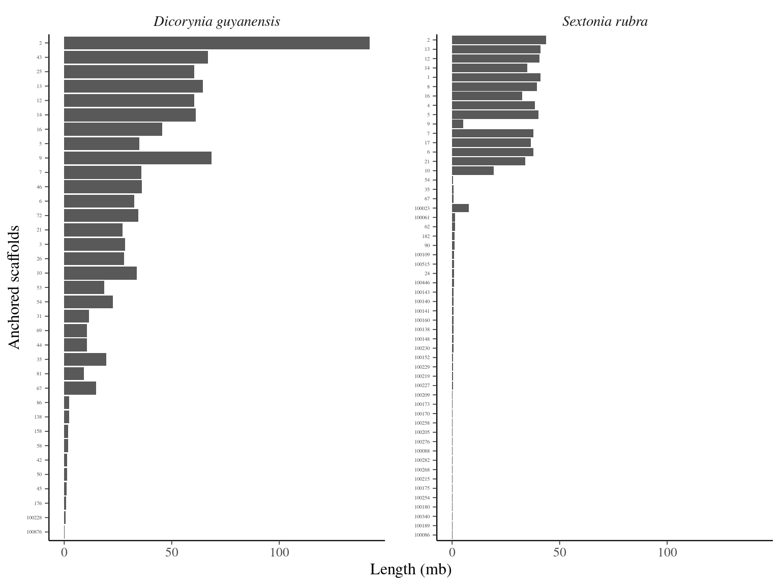
Figure 12.1: Caption.
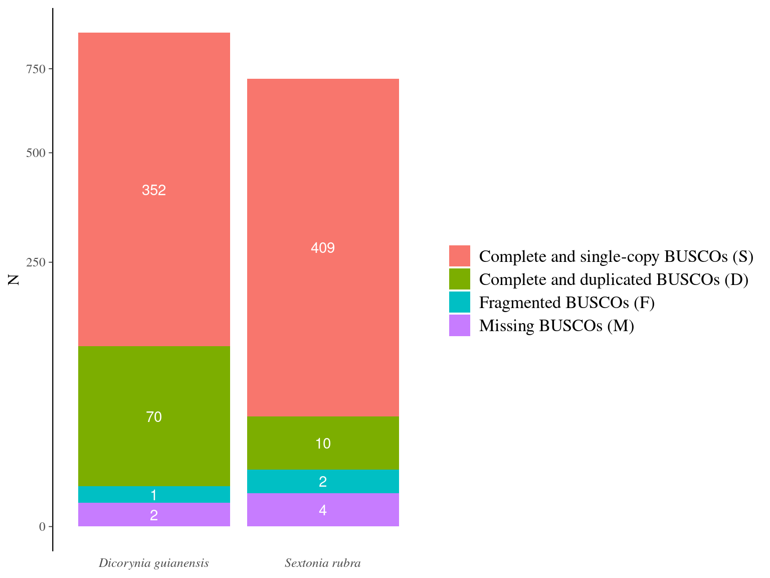
Figure 12.2: Caption.
12.2 Libraries
As expected, Angela’s sequencing depth is twice as high as Sixto’s, averaging about 150X versus 80X (Fig. 12.3), which translates into greater accepted sequencing depth in Angela (note that as a result, Sixto’s libraries are less filtered in terms of coverage, Fig. 12.4).
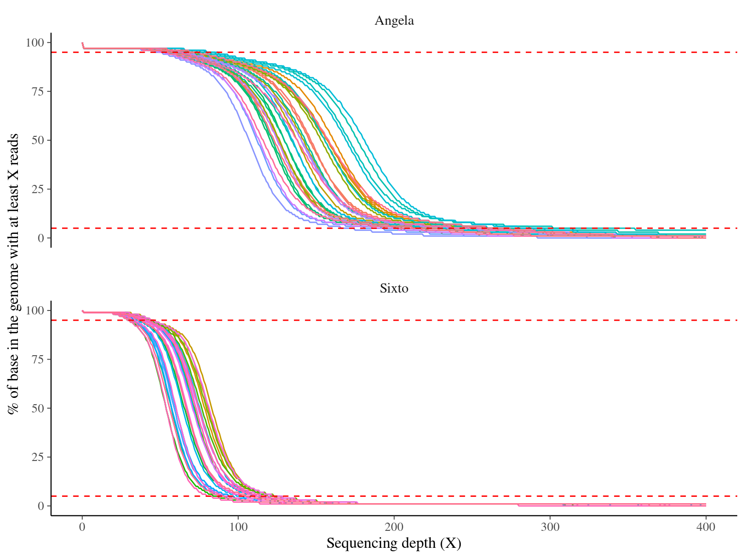
Figure 12.3: Caption.
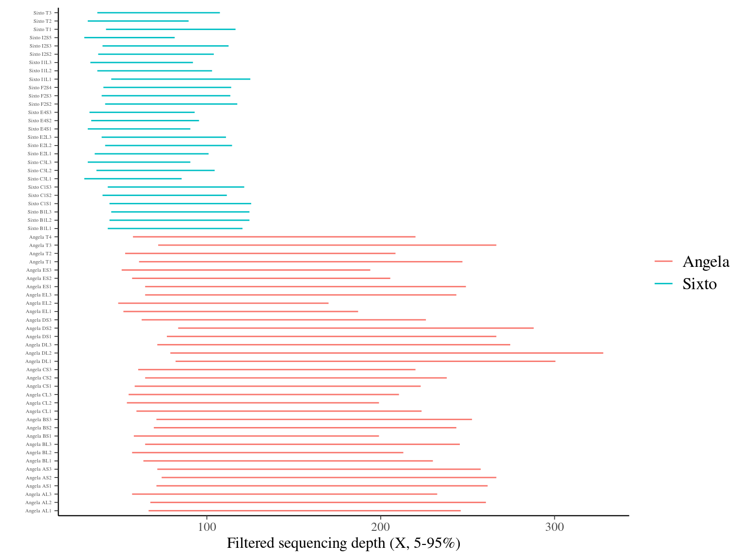
Figure 12.4: Caption.
12.3 Mutations
The origins of the mutations are distributed in the crown, but most of the mutations with basic filtering come from the base of the crown, followed by the carpenter, the branches and finally the tips (Fig. 12.5). Interestingly, stronger filtering favoured mutations in the tips as well as at the base of the crown.
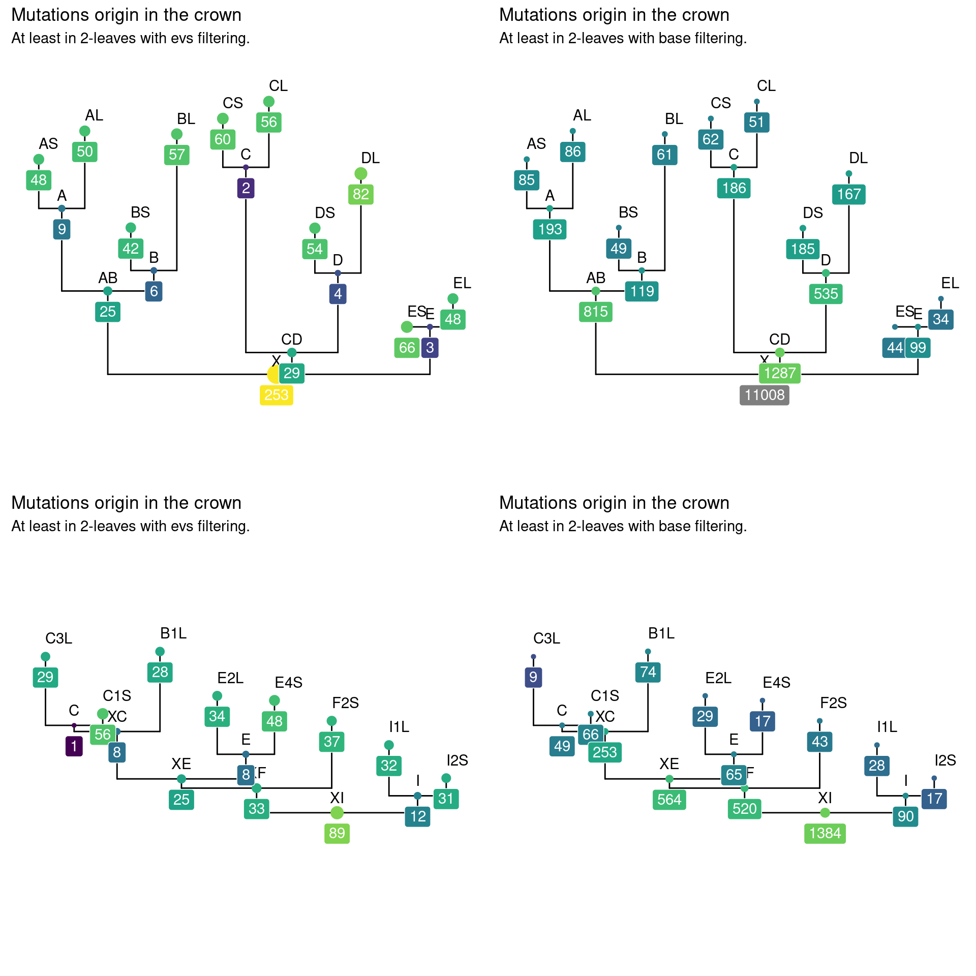
Figure 12.5: Caption.
12.4 Frequencies
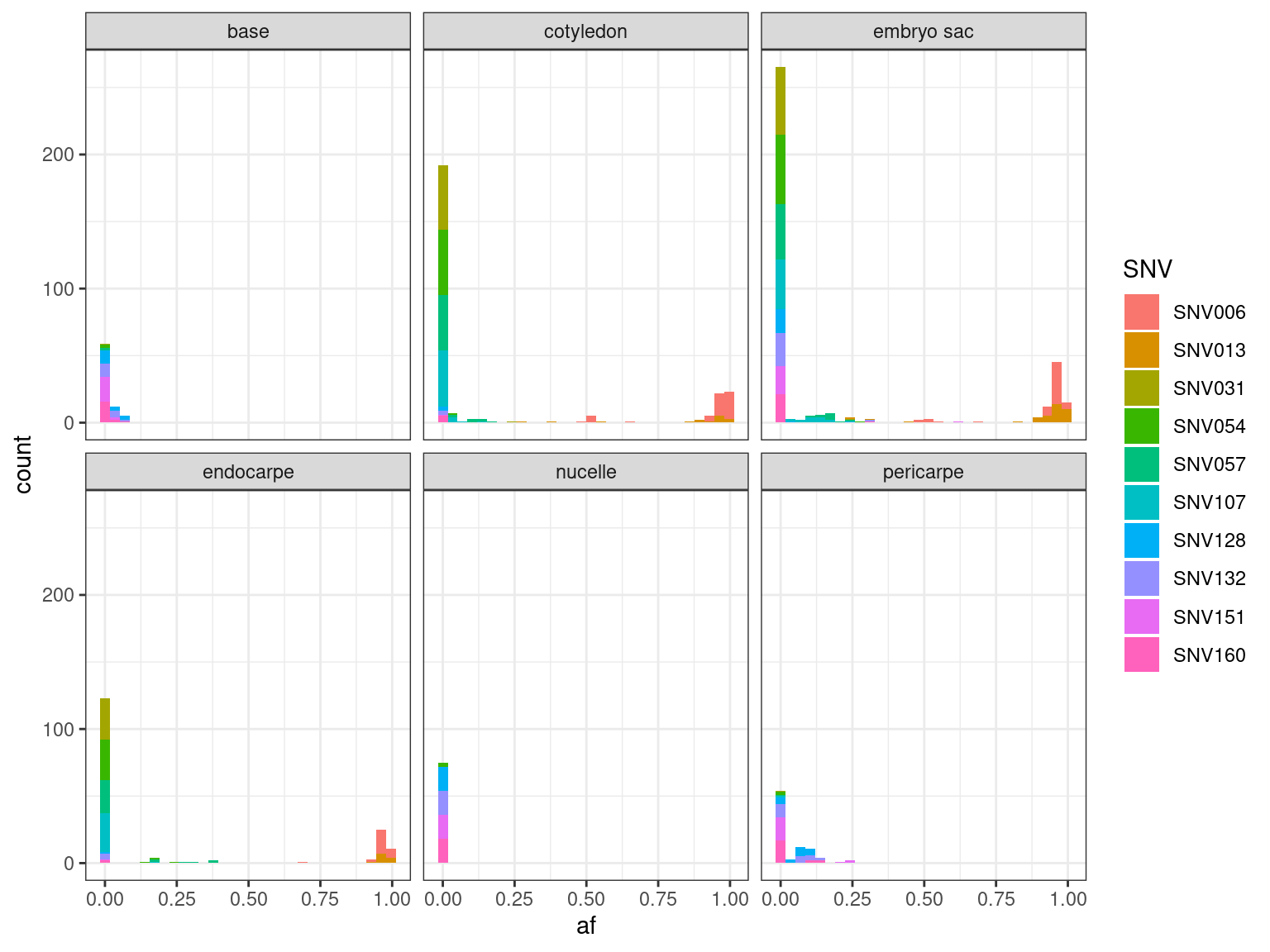
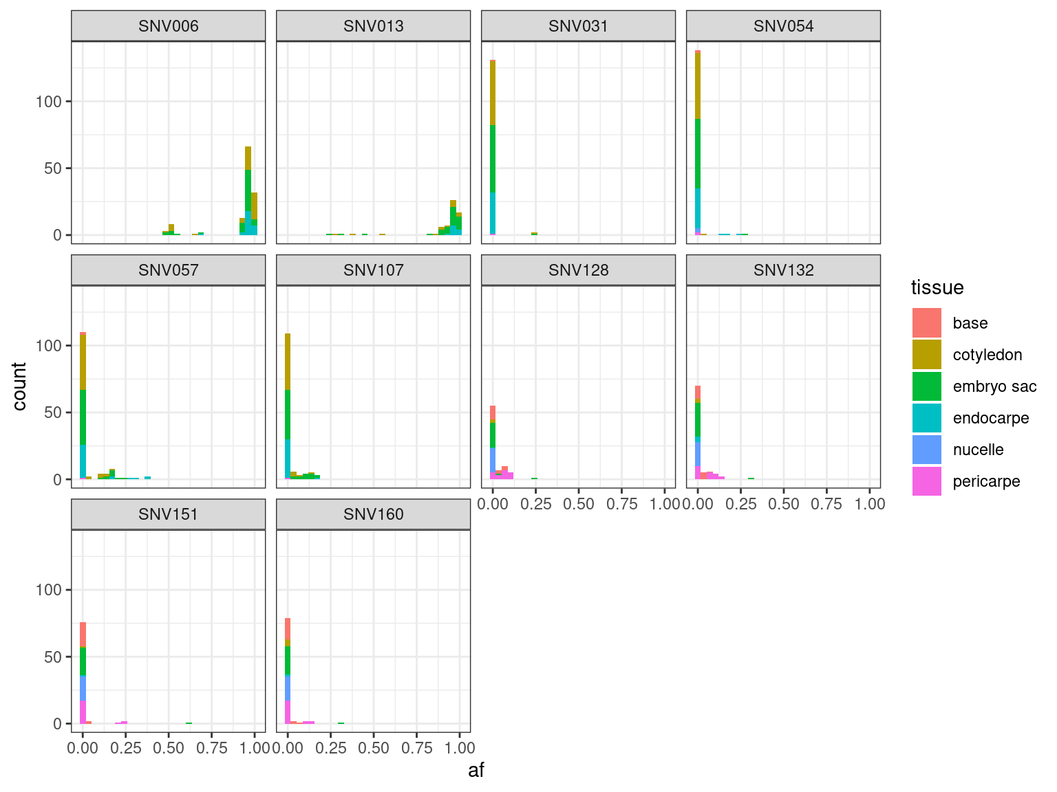
Surprisingly, the allelic frequencies of mutations occurring at the base of the crown are not significantly higher than those at the tips (Fig. 12.6).
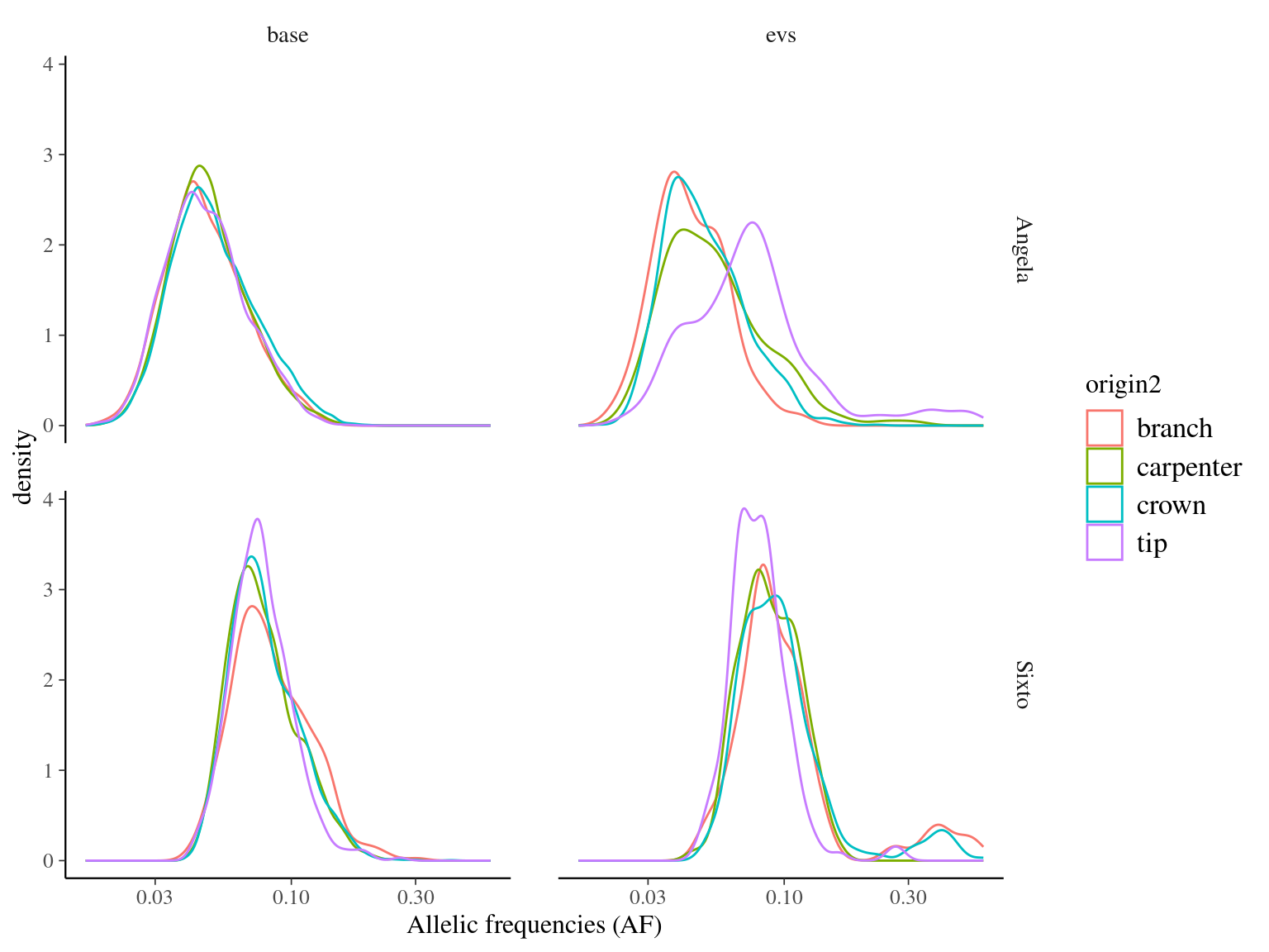
Figure 12.6: Caption.
Figure 12.7: Caption.
Figure 12.8: Caption.
12.5 Phylogeny
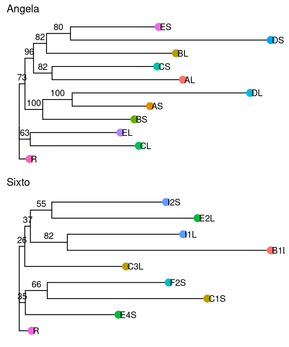
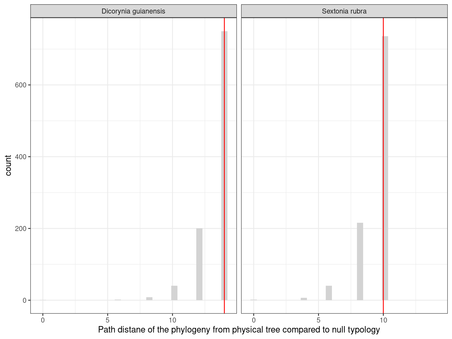
Therefore, mutations are strongly shared across the crown and do not always follow the architecture. As a result, the phylogeny of the mutations does not match the architecture of the tree, with the exception of branch I, which is conserved in Sixto (Fig. 12.9 & Fig. ??).
##
## Setting initial dates...
## Fitting in progress... get a first set of estimates
##          (Penalised) log-lik = -6.362752
## Optimising rates... dates... -6.362752
## Optimising rates... dates... -6.361982
##
## log-Lik = -6.306181
## PHIIC = 66.66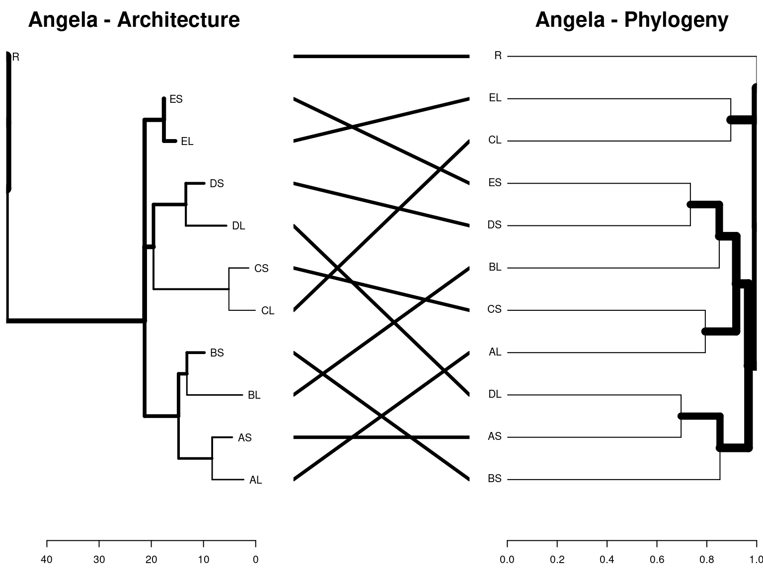
Figure 12.9: Caption.
12.6 Light
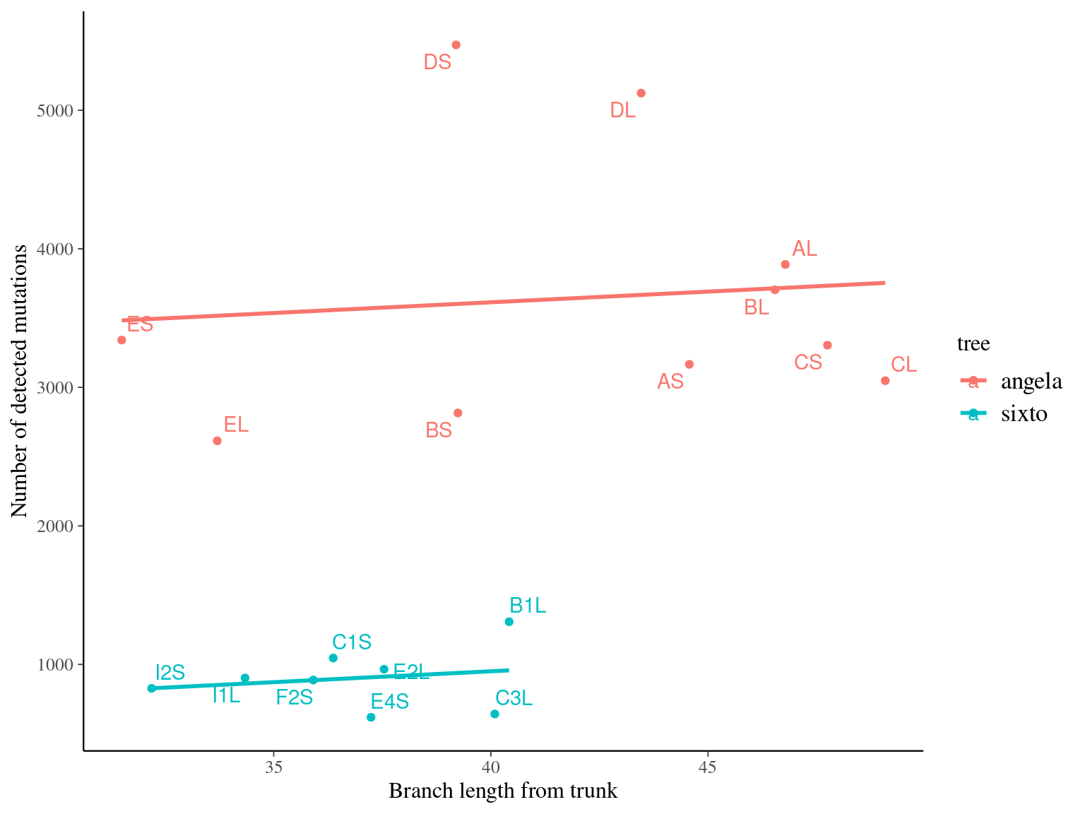
The light condition of the sampled tips at the time of sampling did not affect the number of mutations observed per library (Fig. ??).
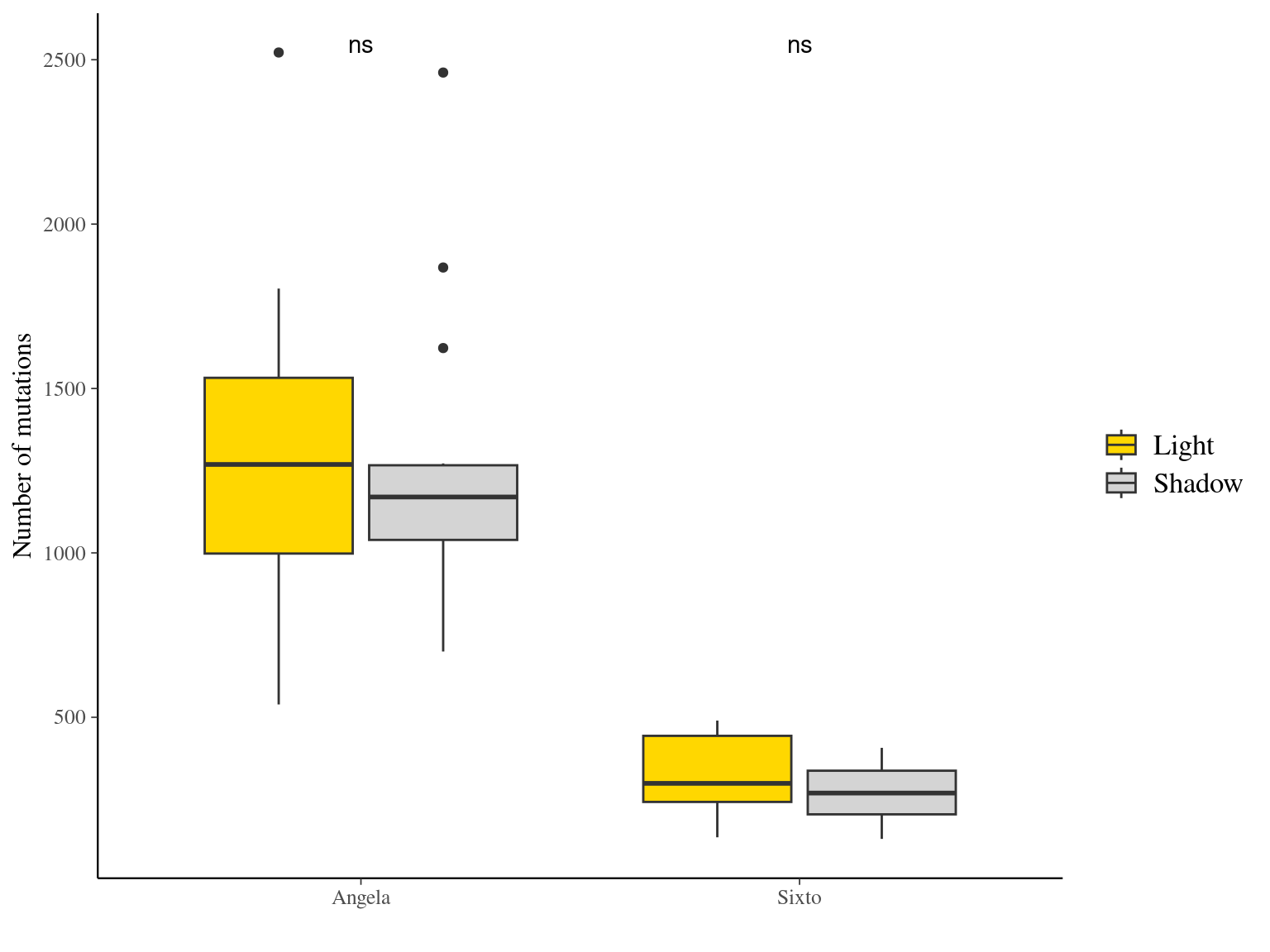
Figure 12.10: Caption.
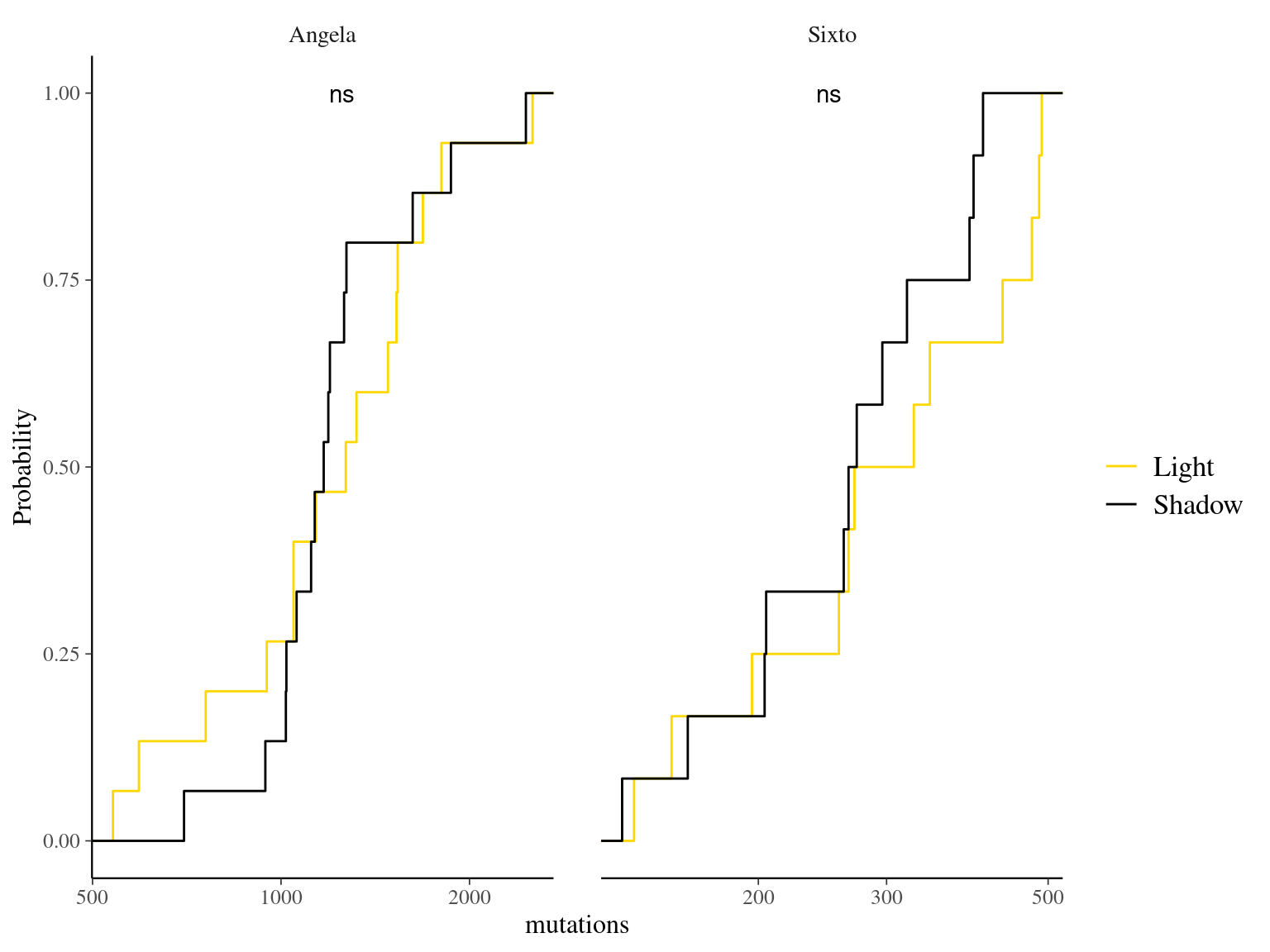
Figure 12.11: Caption.
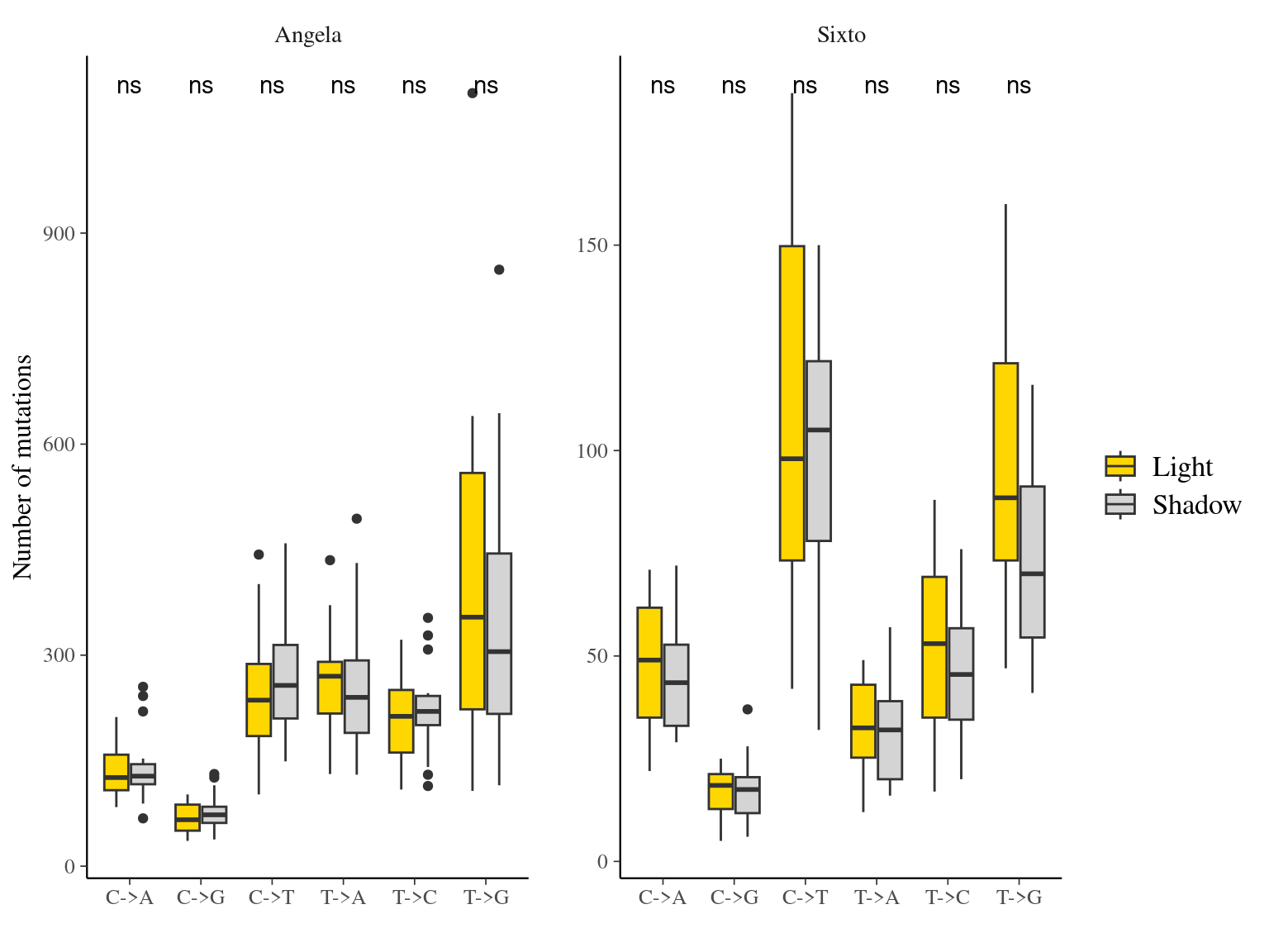
Figure 12.12: Caption.
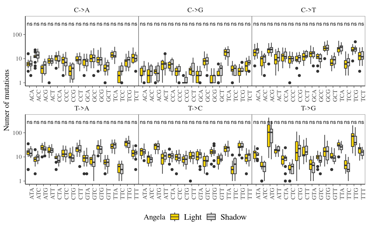
Figure 12.13: Caption.
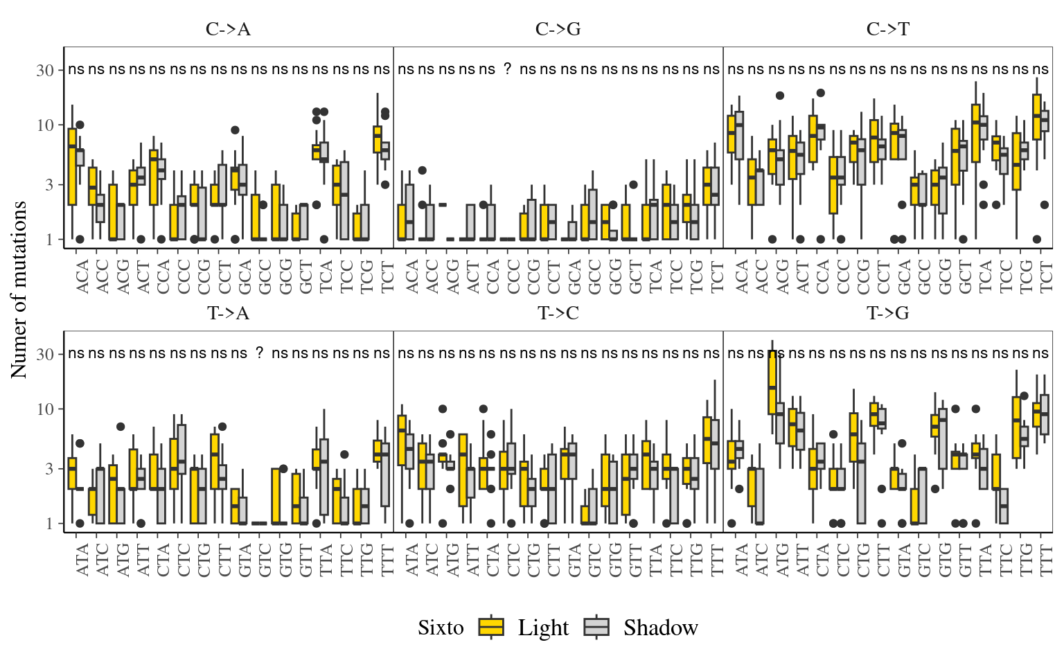
Figure 12.14: Caption.
12.7 Type
Mutation types are similar between Angela and Sixto, with the exception of an increase in C->A and C->T but a decrease in T->A in Sixto compared to Angela, which are probably due to the sampling effect (Fig. 12.15, to be further investigated).
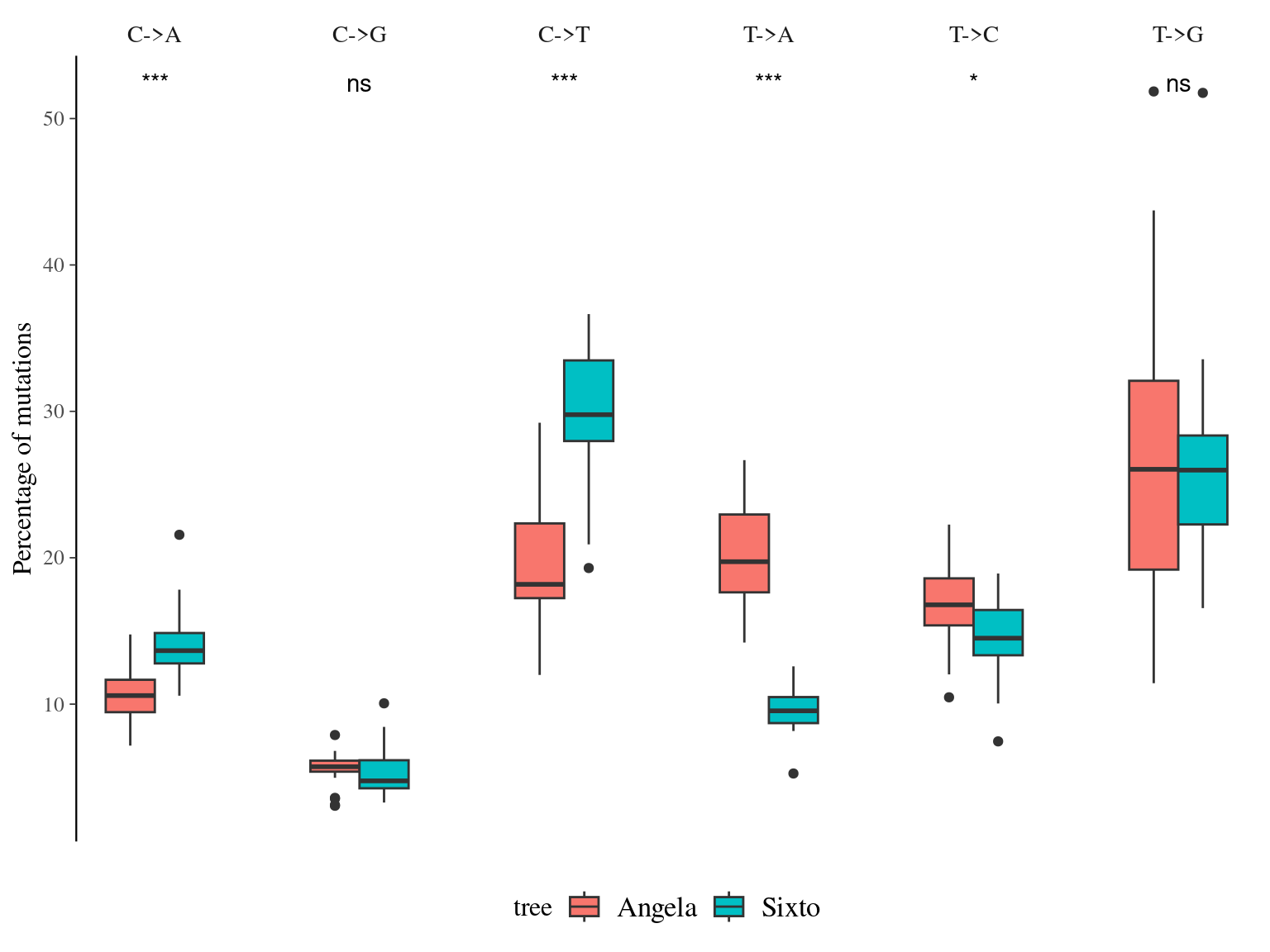
Figure 12.15: Caption.
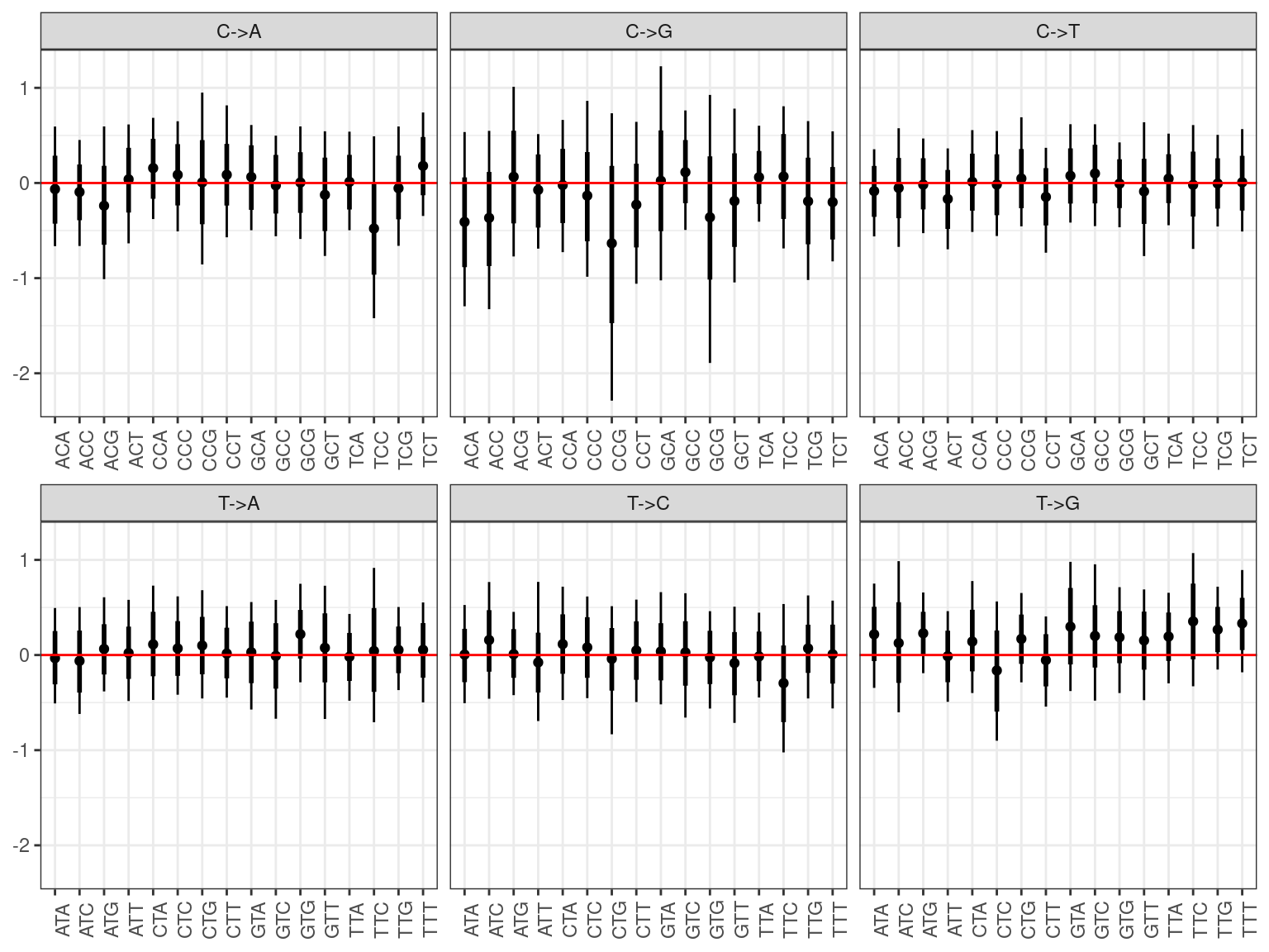
12.8 Spectra
The mutation spectra are similar between Angela and Sixto, with a few exceptions that are probably due to a sampling effect (Fig. 12.16, to be explored further).
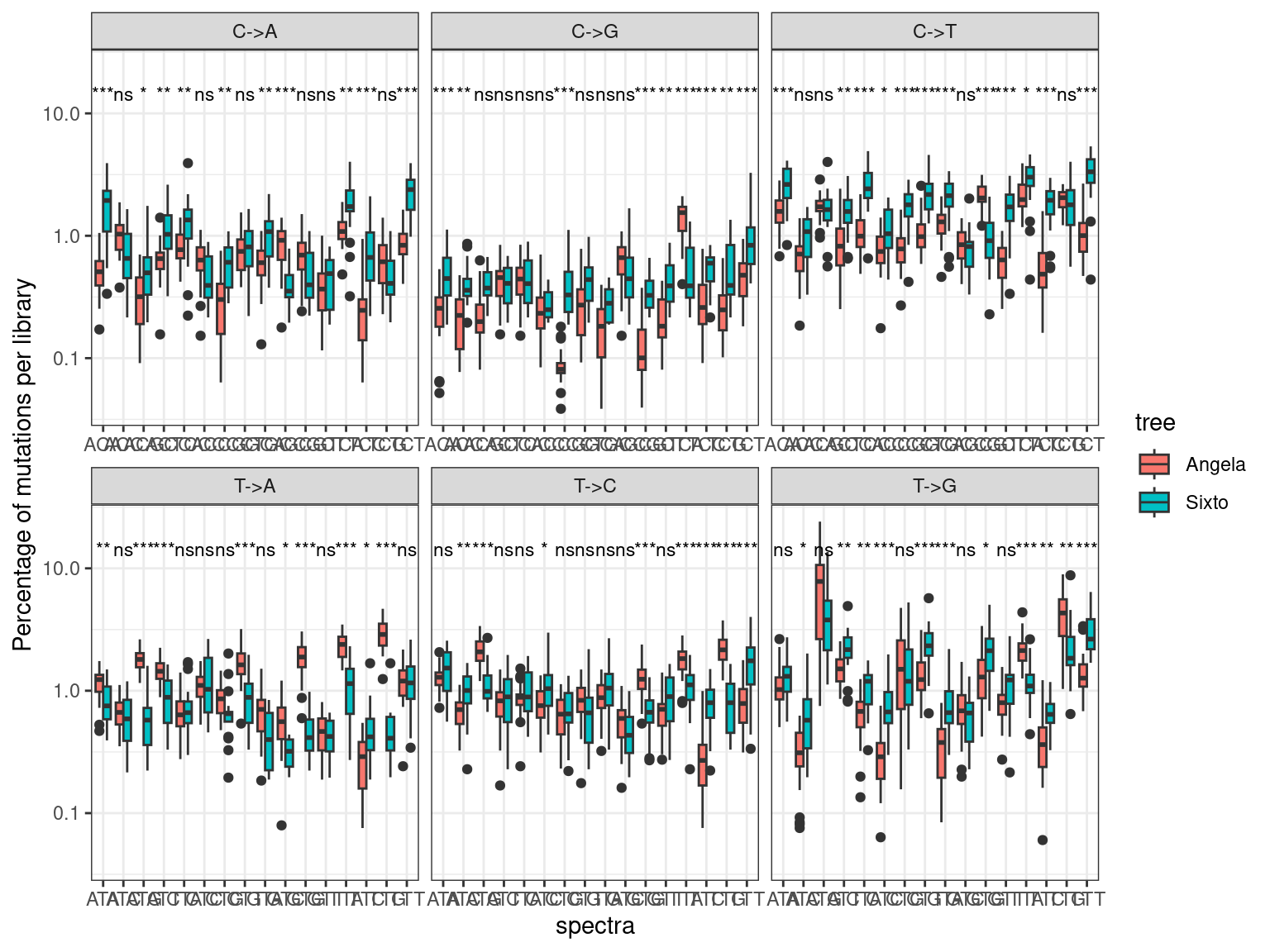
Figure 12.16: Caption.
12.9 Rates
Angela and Sixto show ten to ten thousand mutations depending on the filtering and the minimum accepted allelic frequency (Fig. 12.17). Using base filtering, Angela has a higher number of mutations than Sixto, due to the twofold sequencing depth. Nevertheless, ev filtering gave a similar number of mutations close to thousands in both trees.
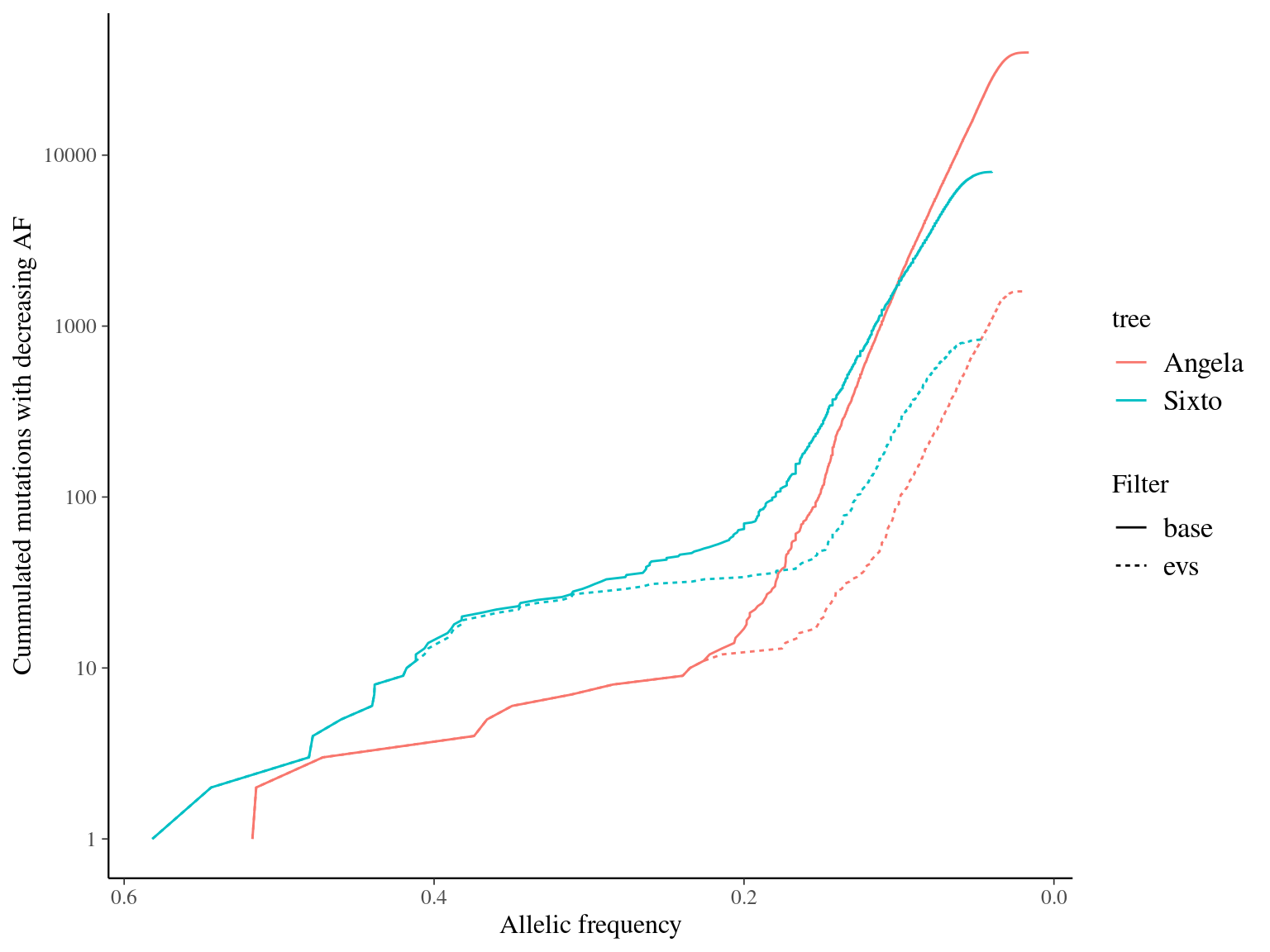
Figure 12.17: Caption.
12.11 Genes
In progress.
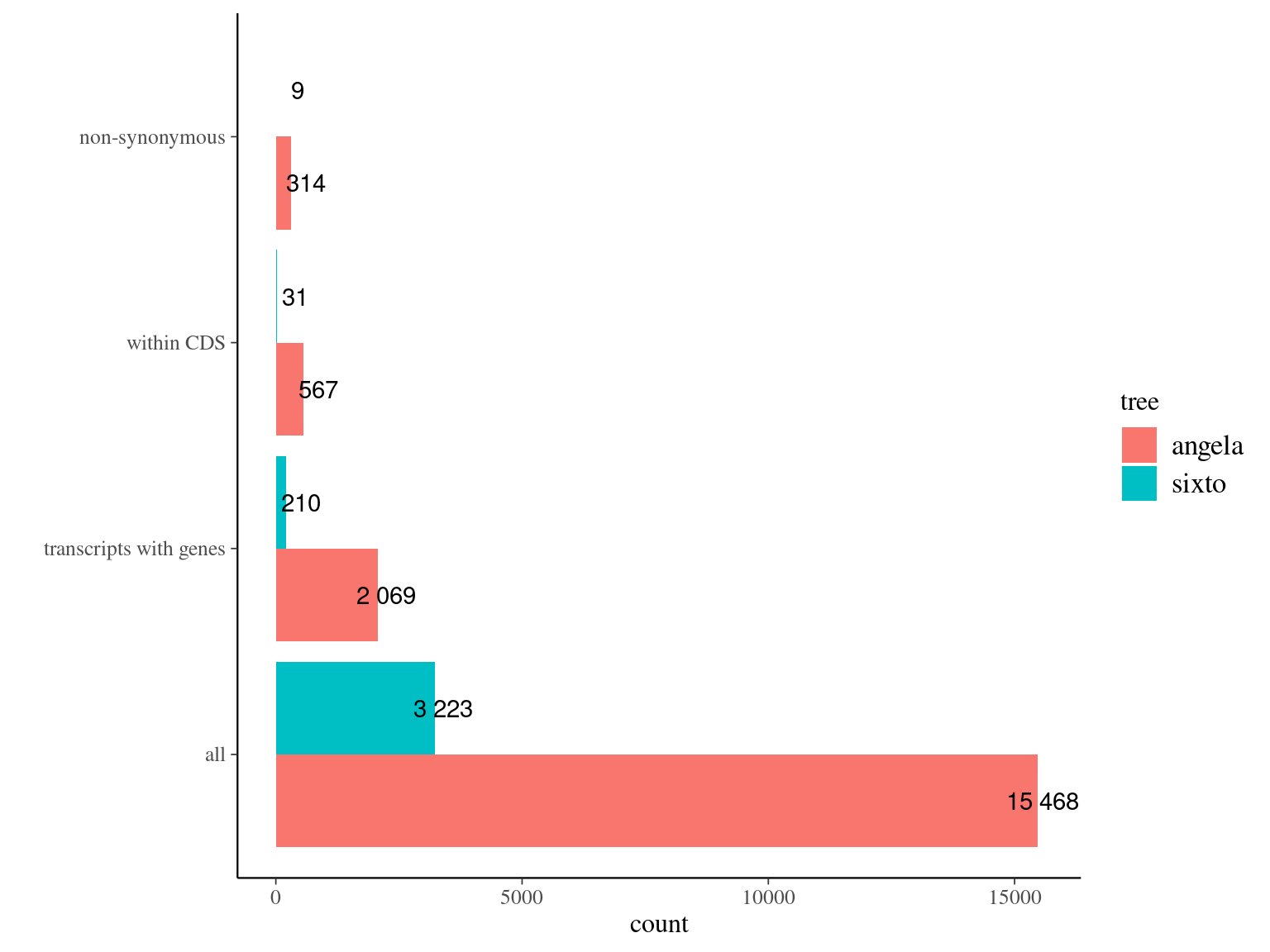
##               Df Sum Sq Mean Sq F value   Pr(>F)
## tree           1  15.52  15.522   87.89  < 2e-16 ***
## synonymy       1  10.63  10.633   60.20 1.47e-14 ***
## Residuals   1698 299.90   0.177
## ---
## Signif. codes:  0 '***' 0.001 '**' 0.01 '*' 0.05 '.' 0.1 ' ' 1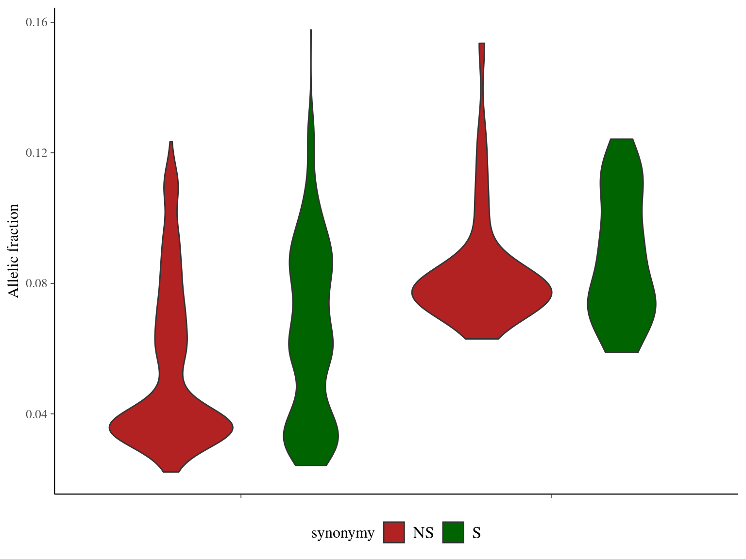
12.12 Fruits
12.12.1 From SSRseq Olivier
12.12.1.1 Align genotypes
library(Biostrings)
candidates <- bind_rows(
  read_tsv("data/mutations/fruits/angela_fruits_candidate_mutations.tsv") %>%
    mutate(mutation = 1:n(), tree = "Angela"),
  read_tsv("data/mutations/fruits/sixto_fruits_candidate_mutations.tsv") %>%
    mutate(mutation = 125:(124+n()), tree = "Sixto")
) %>%
  dplyr::select(CHROM, POS, REF, ALT, af, branch, mutation, tree) %>%
  mutate(CHROM = as.numeric(gsub("Super-Scaffold_", "", CHROM)))
alleles <- readxl::read_xlsx("data/mutations/fruits/SSRseq_TreeMutation_DataAnalysis.xlsx", "AlleleInformation") %>%
  dplyr::rename(locus = Locus, genotype = AlleleSeqCode, sequence = AlleleSequence) %>%
  dplyr::select(locus, genotype, sequence) %>%
  mutate(locus2 = gsub("TreeMut_SNP-", "", locus)) %>%
  separate(locus2, c("mutation", "pos"), "_Super-Scaffold_", convert = T) %>%
  separate_rows(mutation, convert = T) %>%
  separate(pos, "CHROM", convert = T) %>%
  left_join(candidates) %>%
  mutate(name = paste0("SNV", sprintf("%03d", mutation), "_A", genotype))
angela_alleles <- DNAStringSet(filter(alleles, tree == "Angela")$sequence)
names(angela_alleles) <- filter(alleles, tree == "Angela")$name
writeXStringSet(angela_alleles, "data/mutations/fruits/angela_alleles.fa")
sixto_alleles <- DNAStringSet(filter(alleles, tree == "Sixto")$sequence)
names(sixto_alleles) <- filter(alleles, tree == "Sixto")$name
writeXStringSet(sixto_alleles, "data/mutations/fruits/sixto_alleles.fa")
refs <- bind_rows(readxl::read_xlsx("data/mutations/fruits/treemutation_fruits.xlsx", "Sixto") %>%
            mutate(tree = "Sixto"),
          readxl::read_xlsx("data/mutations/fruits/treemutation_fruits.xlsx", "Angela") %>%
            mutate(tree = "Angela")) %>%
  mutate(library = paste0(Code_Espece, Tube), tissue = Tissu) %>%
  dplyr::select(library, tree, tissue) %>%
  bind_rows(readxl::read_xlsx("data/mutations/fruits/Angela.xlsx", "libraries") %>%
              mutate(tissue = paste("branch", branch), library = idOld, tree = "Angela") %>%
              dplyr::select(library, tree, tissue)) %>%
  bind_rows(readxl::read_xlsx("data/mutations/fruits/Sixto.xlsx", "samples") %>%
              mutate(tissue = paste("branch", Branch), library = id, tree = "Sixto") %>%
              dplyr::select(library, tree, tissue))
bwa mem -t 2 ../angela/genome/Dgu_HS1_HYBRID_SCAFFOLD.fa angela_alleles.fa | samtools sort > angela_alleles_aligned.bam
samtools index angela_alleles_aligned.bam
bwa mem -t 2 ../sixto/genome/HS1_Sru_omap1_hap1_HYBRID_SCAFFOLD.fa sixto_alleles.fa | samtools sort > sixto_alleles_aligned.bam
samtools index sixto_alleles_aligned.bam12.12.1.2 Automate IGV
conda create -n igvreports python=3.7.1
conda activate igvreports
pip install igv-reports
conda deactivate
conda activate igvreports
create_report data/mutations/fruits/angela_fruits_candidate_mutations.tsv \
data/mutations/angela/genome/Dgu_HS1_HYBRID_SCAFFOLD.fa \
--sequence 2 --begin 3 --end 3 \
--flanking 1000 \
--info-columns SNV CHROM POS REF ALT af replicate branch rank \
--tracks data/mutations/fruits/angela_alleles_aligned.bam data/mutations/angela/annotation/Dgu_HS1_HYBRID_SCAFFOLD.fa.out.gff \
--output data/mutations/fruits/angela_fruits_aligned.html
conda deactivateconda activate igvreports
create_report data/mutations/fruits/sixto_fruits_candidate_mutations.tsv \
data/mutations/sixto/genome/HS1_Sru_omap1_hap1_HYBRID_SCAFFOLD.fa \
--sequence 2 --begin 3 --end 3 \
--flanking 1000 \
--info-columns SNV CHROM POS REF ALT af replicate branch rank \
--tracks data/mutations/fruits/sixto_alleles_aligned.bam data/mutations/sixto/annotation/HS1_Sru_omap1_hap1_HYBRID_SCAFFOLD.fa.out.gff \
--output data/mutations/fruits/sixto_fruits_aligned.html
conda deactivate12.12.1.3 Results
##             Type Angela Sixto Total Percentage
## 1       mutation     16     5    21         15
## 2 reference only     81    20   101         72
## 3        suspect     11     6    17         12
## 4 unaligned 16 5 21 15pdf( "data/mutations/fruits/fruits_mutations.pdf")
for(i in 1:ggforce::n_pages(graph))
print(graph + ggforce::facet_wrap_paginate(~title, scales = "free",
ncol = 1, nrow = 1, page = i))
dev.off()
12.12.1.4 Tissues
| SNV | FALSE | TRUE | agreement |
|---|---|---|---|
| SNV006 | 0 | 52 | 100 |
| SNV013 | 0 | 50 | 100 |
| SNV031 | 0 | 52 | 100 |
| SNV054 | 1 | 51 | 98 |
| SNV057 | 8 | 44 | 85 |
| SNV107 | 6 | 46 | 88 |
| SNV128 | 0 | 19 | 100 |
| SNV132 | 0 | 19 | 100 |
| SNV151 | 0 | 20 | 100 |
| SNV160 | 0 | 19 | 100 |
| fruit | cotyledon | embryo sac |
|---|---|---|
| A1 | NA | homozygous |
| A10 | homozygous | homozygous |
| A11 | homozygous | homozygous |
| A12 | homozygous | heterozygous |
| A13 | homozygous | homozygous |
| A14 | homozygous | homozygous |
| A15 | heterozygous | heterozygous |
| A16 | homozygous | homozygous |
| A17 | NA | homozygous |
| A18 | homozygous | heterozygous |
| A19 | homozygous | homozygous |
| A2 | homozygous | homozygous |
| A20 | homozygous | homozygous |
| A3 | homozygous | homozygous |
| A4 | homozygous | homozygous |
| A5 | homozygous | heterozygous |
| A6 | homozygous | heterozygous |
| A7 | homozygous | homozygous |
| A8 | homozygous | homozygous |
| A9 | homozygous | homozygous |
| B1 | homozygous | homozygous |
| B10 | homozygous | homozygous |
| B11 | homozygous | homozygous |
| B12 | homozygous | homozygous |
| B13 | homozygous | homozygous |
| B14 | homozygous | homozygous |
| B15 | homozygous | homozygous |
| B16 | homozygous | heterozygous |
| B17 | homozygous | homozygous |
| B18 | homozygous | heterozygous |
| B19 | heterozygous | heterozygous |
| B2 | homozygous | homozygous |
| B20 | homozygous | homozygous |
| B21 | homozygous | homozygous |
| B22 | homozygous | homozygous |
| B23 | homozygous | NA |
| B24 | homozygous | homozygous |
| B25 | homozygous | homozygous |
| B3 | homozygous | homozygous |
| B4 | homozygous | homozygous |
| B5 | homozygous | heterozygous |
| B6 | homozygous | homozygous |
| B7 | homozygous | homozygous |
| B8 | homozygous | homozygous |
| B9 | homozygous | homozygous |
| C1 | NA | homozygous |
| C2 | homozygous | homozygous |
| C3 | homozygous | homozygous |
| D1 | homozygous | homozygous |
| D2 | homozygous | homozygous |
| D3 | homozygous | heterozygous |
| D5 | NA | homozygous |
| SNV | cotyledon | embryo sac | endocarpe | pericarpe |
|---|---|---|---|---|
| SNV006 | 7 | 7 | 1 | NA |
| SNV013 | 2 | 3 | NA | NA |
| SNV031 | NA | 1 | NA | NA |
| SNV054 | NA | 1 | 3 | NA |
| SNV057 | 2 | 10 | 6 | NA |
| SNV107 | 1 | 6 | 1 | NA |
| SNV128 | NA | 1 | NA | NA |
| SNV132 | NA | 1 | NA | 2 |
| SNV151 | NA | 1 | NA | 3 |
| SNV160 | NA | 1 | NA | 3 |