Inventories

Inventory data from Paracou, including understory trees, and Tapajos were used both as input to the TROLL assessment for the species list and as output to assess forest structure, neutral composition and species list.

Code

tapajos <- read_csv("data/inventories/data/Tapajos_inventory_data_2010.csv", na = "-9999") %>% 
  filter(type == "PF") %>% 
  separate(scientific_name, c("genus", "species")) %>% 
  mutate(species = paste(genus, species), wsg = density_wood, h = ht_total) %>% 
  mutate(site = "Tapajos", type = "default", x = stem_x, y = stem_y) %>% 
  filter(dbh >= 10) %>% 
  select(site, type, plot, tree, species, dbh, x, y) %>% 
  mutate(plot_size = 0.25)
paracou <- read_tsv("data/inventories/guyafor.tsv") %>% 
  filter(Forest == "Paracou") %>% 
  mutate(plot = as.numeric(Plot)) %>% 
  filter(!is.na(plot)) %>% 
  filter(Plot != 16) %>% 
  filter(Plot %in% c(1, 6, 11, 13:15)) %>% 
  filter(BotaSource == "Bota") %>% 
  filter(!is.na(Xutm), !is.na(Yutm)) %>% 
  filter(CodeAlive == 1) %>% 
  mutate(dbh = CircCorr/pi, site = "Paracou", type = "default", tree = idTree,
         x = Xfield, y = Yfield) %>% 
  filter(CensusYear == 2005) %>% 
  filter(dbh >= 10) %>% 
  separate(Species, "Species") %>% 
  mutate(species = paste(Genus, Species), plot_size = PlotArea) %>% 
  select(site, type, plot, tree, species, dbh, x, y, plot_size)
paracou_understory <- read_csv("data/inventories/understory_paracou_9ha_20231119.csv") %>% 
  mutate(plot = subplot) %>% 
  mutate(dbh = DBH, site = "Paracou", type = "understory", tree = TreeID, x = X, y = Y) %>% 
  filter(dbh <= 10) %>% 
  select(site, type, plot, tree, species, dbh, x, y) %>% 
  mutate(tree = as.numeric(as.factor(tree))) %>% 
  mutate(plot_size = 1)
bind_rows(paracou, paracou_understory, tapajos) %>% 
  write_tsv("outputs/inventories.tsv")
read_tsv("outputs/inventories.tsv") %>% 
  mutate(plot = ifelse(site == "Tapajos", 1, plot)) %>% 
  mutate(plot_size = ifelse(site == "Tapajos", 2, plot_size)) %>% 
  mutate(dbh_class = cut(dbh, 
                         breaks = c(seq(1, 9, by = 1), seq(10, 200, by = 10)), 
                         labels = c(seq(1, 9, by = 1)+0.5, seq(10, 190, by = 10)+5))) %>% 
  mutate(dbh_class = as.numeric(as.character(dbh_class))) %>% 
  group_by(site, type, plot, dbh_class) %>% 
  summarise(abundance = n()/unique(plot_size),
            ba = sum((dbh/2)^2*pi)/10^4/unique(plot_size)) %>% 
  mutate(log_abundance = log10(abundance)) %>% 
  gather(variable, observed, -site, -type, -plot, -dbh_class) %>% 
  write_tsv("outputs/structure.tsv")
read_tsv("outputs/inventories.tsv") %>% 
  mutate(plot = ifelse(site == "Tapajos", 1, plot)) %>% 
  mutate(plot_size = ifelse(site == "Tapajos", 2, plot_size)) %>% 
  filter(type == "default") %>% 
  group_by(site, plot, species) %>% 
  summarise(observed = n()/plot_size) %>% 
  unique() %>% 
  mutate(variable = "abundance") %>% 
  write_tsv("outputs/composition.tsv")

Paracou

Paracou is a large scale forest disturbance experiment set up by Cirad in 1982 that becomes in time a unique research site for the international scientific community in tropical forest ecology. https://paracou.cirad.fr/website/

PI: Géraldine Derroire

Access: DOIs are available on the CIRAD dataverse: https://dataverse.cirad.fr/dataverse/paracou .

Code

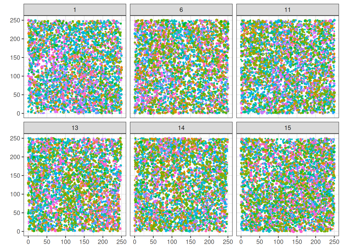
read_tsv("outputs/inventories.tsv", show_col_types = FALSE) %>% 
  filter(site == "Paracou", type == "default") %>% 
  ggplot(aes(x, y, size = dbh, col = species)) +
  geom_point() +
  facet_wrap(~ plot) +
  scale_color_discrete(guide = "none") +
  theme_bw() +
  theme(axis.title = element_blank()) +
  scale_size(guide = "none", range = c(0.2, 2)) +
  coord_equal()

Tree distributions in the 2015 inventory of Paracou plots. Point size represents the diameter, and the colour the species.

Paracou - Understory

Forest plots in French Guiana (Paracou and Nouragues) and inventory and map all trees over one cm in height at the chest, in order to advance knowledge of the ecology and services of the Amazon ecosystem.

PIs: Giacomo Sellan, Gérladine Derroire, Jérôme Chave

Access: Upon request?

Code

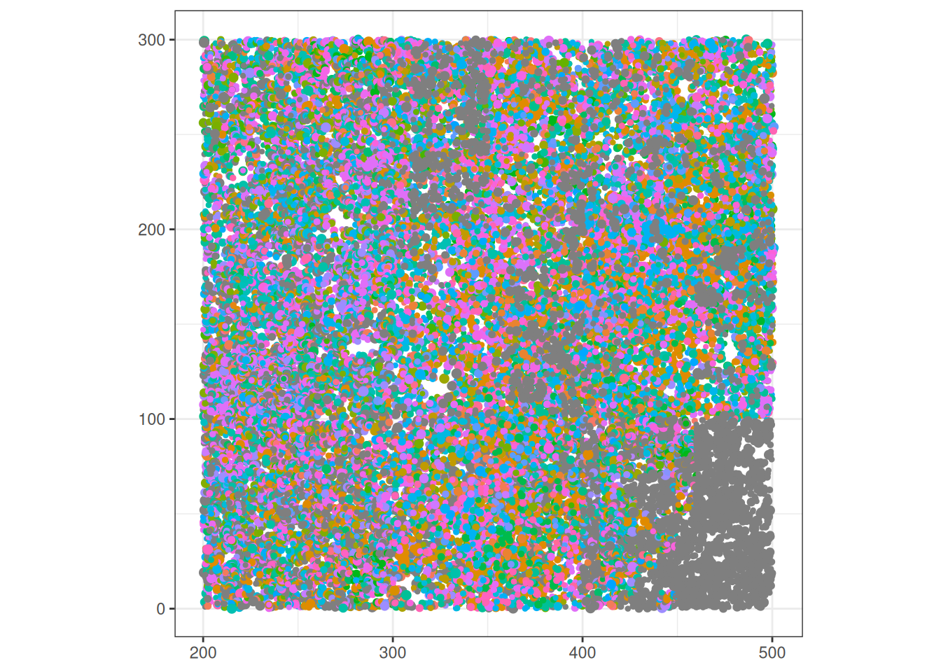
read_tsv("outputs/inventories.tsv", show_col_types = FALSE) %>% 
  filter(site == "Paracou", type == "understory") %>% 
  filter(!is.na(x), !is.na(y)) %>% 
  ggplot(aes(x, y, size = dbh, col = species)) +
  geom_point() +
  scale_color_discrete(guide = "none") +
  theme_bw() +
  theme(axis.title = element_blank()) +
  scale_size(guide = "none", range = c(0.2, 2)) +
  coord_equal()

Tree distributions in the Understory inventory at Paracou. Point size represents the diameter, and the colour the species.

Tapajos

This dataset provides tree inventory, tree height, diameter at breast height (DBH), and estimated crown measurements from 30 plots located in the Tapajos National Forest, Para, Brazil collected in September 2010. The plots were located in primary forest, primary forest subject to reduced-impact selective logging (PFL) between 1999 and 2003, and secondary forest (SF) with different age and disturbance histories. Plots were centered on GLAS (the Geoscience Laser Altimeter System) LiDAR instrument footprints selected along two sensor acquisition tracks spanning a wide range in vertical structure and aboveground biomass. https://daac.ornl.gov/VEGETATION/guides/Forest_Inventory_Tapajos.html

Access: These data are available through the Oak Ridge National Laboratory (ORNL) Distributed Active Archive Center (DAAC).

Code

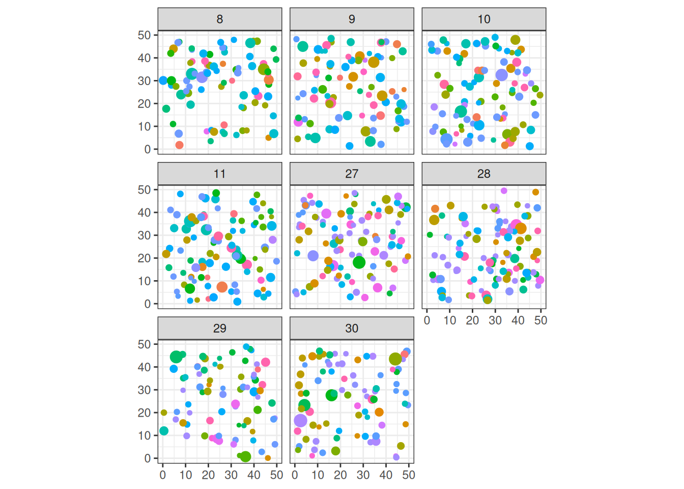
read_tsv("outputs/inventories.tsv", show_col_types = FALSE) %>% 
  filter(site == "Tapajos", type == "default") %>% 
  ggplot(aes(x, y, size = dbh, col = species)) +
  geom_point() +
  facet_wrap(~ plot) +
  scale_color_discrete(guide = "none") +
  theme_bw() +
  theme(axis.title = element_blank()) +
  scale_size(guide = "none", range = c(1, 4)) +
  coord_equal()

Tree distributions in the inventory of Tapajos plots. Point size represents the diameter, and the colour the species.

Airborne Lidar Scanning (ALS)

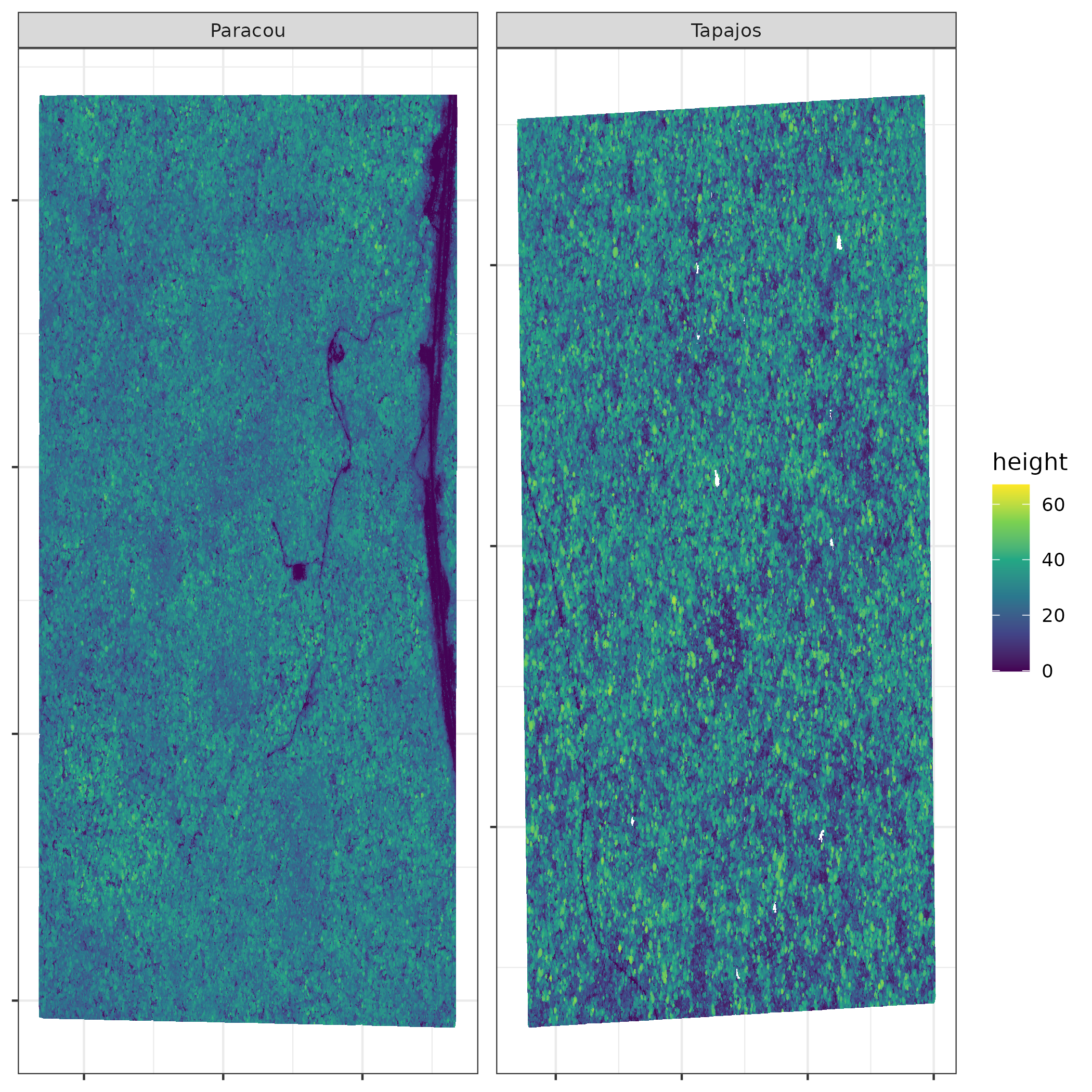
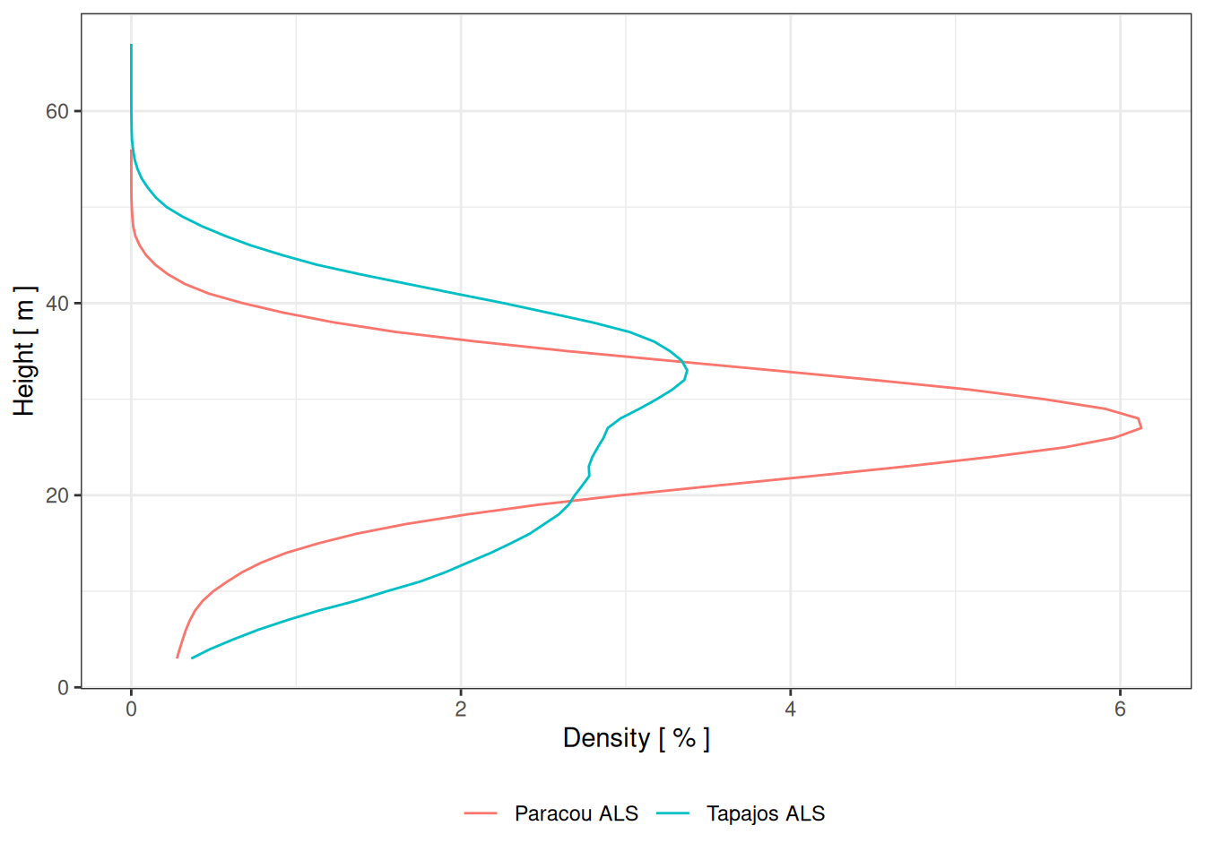
We evaluated tree height distributions using ALS data from 2015 at Paracou (unpublished data) and from 2012 at Tapajos (dos-Santos et al., 2019), which were processed into canopy height models with a standardised pipeline (Fischer et al., 2024). From both simulated and ALS-derived canopy height models, we derived the distribution of canopy height, expressed in proportion of 1-m2 pixels per 1-m height class.

Code

paracou <- rast("data/inventories/chm/chm_lspikefree_paracou2015.tif") %>% 
  # crop(ext(285000,286000,581500,582500)) %>% 
  as.data.frame(xy = TRUE) %>% 
  mutate(site = "Paracou") %>% 
  rename(height = spat_UnJH55x5kyQCEFH_27216)
tapajos <- rast("data/inventories/chm/chm_lspikefree_tapajos2012.tif") %>% 
  # crop(ext(727000,728000,9683000,9684000)) %>% 
  as.data.frame(xy = TRUE) %>% 
  mutate(site = "Tapajos") %>% 
  rename(height = spat_A96aTkDLpl6EakG_7172)
g <- bind_rows(paracou, tapajos) %>% 
  ggplot(aes(x, y, fill = height)) +
  geom_raster() +
  theme_bw() +
  facet_wrap(~site, scales = "free") +
  scale_fill_viridis_c() +
  theme(axis.title = element_blank(), axis.text = element_blank())
ggsave("outputs/chm_fig.png", g)
bind_rows(paracou, tapajos) %>% 
  group_by(site, height = floor(height)) %>% 
  summarise(n = n()) %>% 
  group_by(site) %>% 
  mutate(pct = n/sum(n)*100, type = "ALS") %>% 
  write_tsv("outputs/hieght_chm.tsv")

Code

knitr::include_graphics("outputs/chm_fig.png")

Canpy Height Model (CHM) from Aerial Lidar Sensors (ALS) at Paracou an Tapajos.

Structure

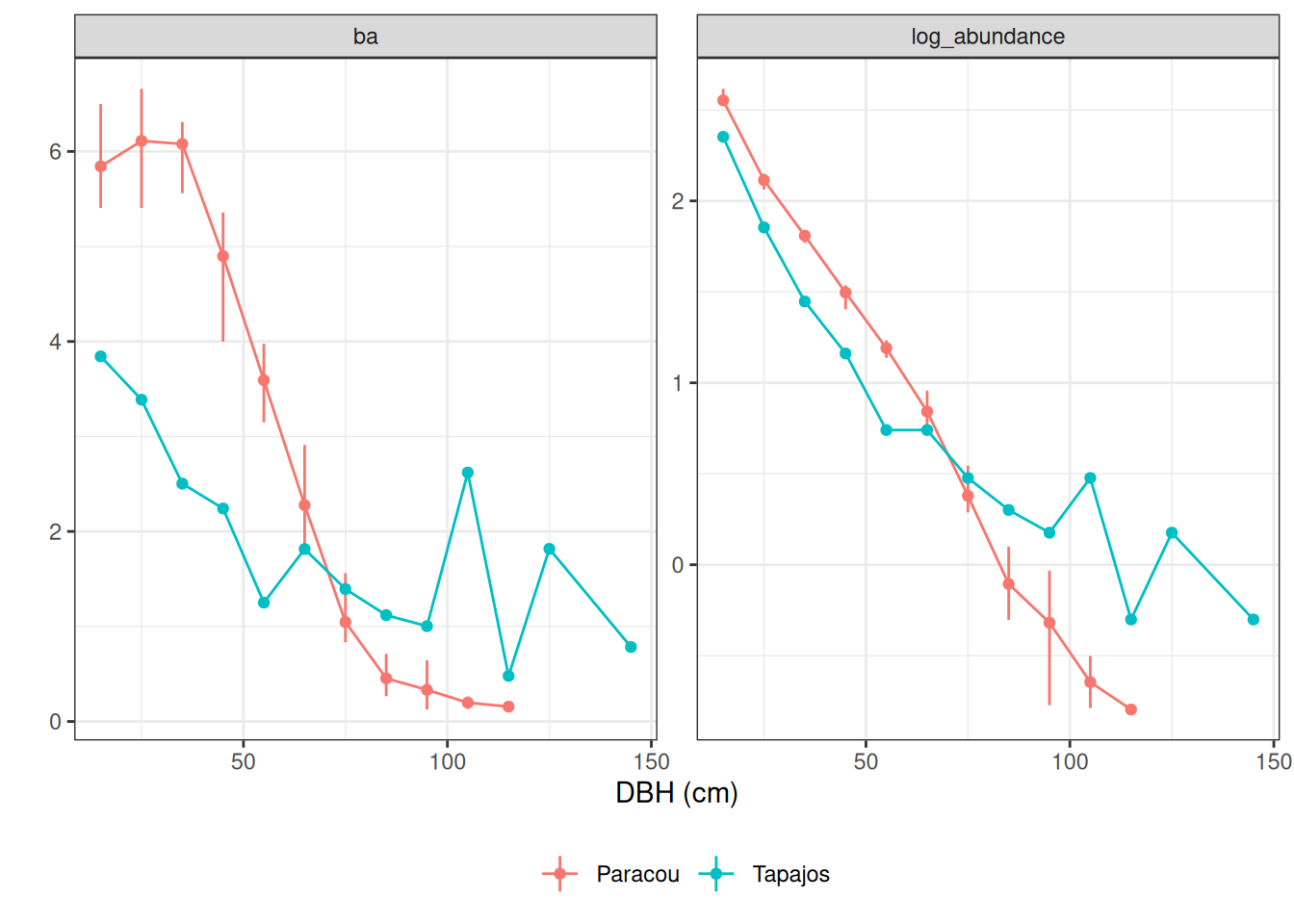
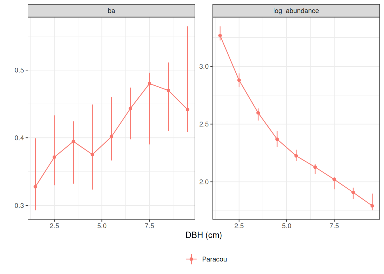
Forest structure was simply assessed by DBH (m) classes using basal area (BA, m2/ha) and number of stems for each plots (uncertainty bars in Paracou data).

Code

read_tsv("outputs/structure.tsv", show_col_types = FALSE) %>% 
  filter(dbh_class >= 10) %>% 
  group_by(site, type, dbh_class, variable) %>% 
  summarise(l = quantile(observed, 0.025, na.rm = TRUE), 
            m = quantile(observed, 0.5, na.rm = TRUE), 
            h = quantile(observed, 0.975, na.rm = TRUE)) %>% 
  filter(variable %in% c("ba", "log_abundance")) %>% 
  ggplot(aes(dbh_class, m, col = site)) +
  geom_linerange(aes(ymin = l, ymax = h)) +
  geom_point() +
  geom_line() +
  theme_bw() +
  facet_wrap(~ variable, scales = "free") +
  xlab("DBH (cm)") + ylab("") +
  scale_color_discrete("") +
  theme(legend.position = "bottom")

Size structure at the Paracou and Tapajos sites, expressed in terms of number of stems and basal area and including understorey trees at Paracou. Confidence intervals on inventory analysis at 95 % are shown with error bars and are based on among plots variations.

Code

read_tsv("outputs/structure.tsv", show_col_types = FALSE) %>% 
  filter(dbh_class < 10) %>% 
  group_by(site, type, dbh_class, variable) %>% 
  summarise(l = quantile(observed, 0.025, na.rm = TRUE), 
            m = quantile(observed, 0.5, na.rm = TRUE), 
            h = quantile(observed, 0.975, na.rm = TRUE)) %>% 
  filter(variable %in% c("ba", "log_abundance")) %>% 
  ggplot(aes(dbh_class, m, col = site)) +
  geom_linerange(aes(ymin = l, ymax = h)) +
  geom_point() +
  geom_line() +
  theme_bw() +
  facet_wrap(~ variable, scales = "free") +
  xlab("DBH (cm)") + ylab("") +
  scale_color_discrete("") +
  theme(legend.position = "bottom")

Size structure at the Paracou and Tapajos sites, expressed in terms of number of stems and basal area and including understorey trees at Paracou. Confidence intervals on inventory analysis at 95 % are shown with error bars and are based on among plots variations.

Code

read_tsv("outputs/hieght_chm.tsv") %>% 
  filter(height > 2) %>% 
  ggplot(aes(height, pct, col = paste(site, type))) +
  geom_line() +
  theme_bw() +
  coord_flip() +
  ylab("Density [ % ]") + xlab("Height [ m ]") +
  theme(legend.position = "bottom") +
  scale_color_discrete("")

Height structure at the Paracou and Tapajos sites.

Composition

Forest composition was simply assessed using rank abundances curves for each plots (uncertainty dotted lines in Paracou data).

Code

read_tsv("outputs/composition.tsv", show_col_types = FALSE) %>% 
  group_by(site, plot, variable) %>% 
  arrange(desc(observed)) %>% 
  mutate(rank = 1:n()) %>% 
  group_by(site, rank, variable) %>% 
  summarise(l = quantile(observed, 0.025, na.rm = TRUE), 
            m = quantile(observed, 0.5, na.rm = TRUE), 
            h = quantile(observed, 0.975, na.rm = TRUE)) %>% 
  ggplot(aes(rank, m, col = site)) +
  geom_line(aes(y = l), linewidth = 0.5, linetype = "dashed") +
  geom_line(aes(y = h), linewidth = 0.5, linetype = "dashed") +
  geom_line() +
  theme_bw() +
  xlab("Rank") + ylab("Abundance") +
  scale_color_discrete("") +
  theme(legend.position = "bottom") +
  scale_y_log10()

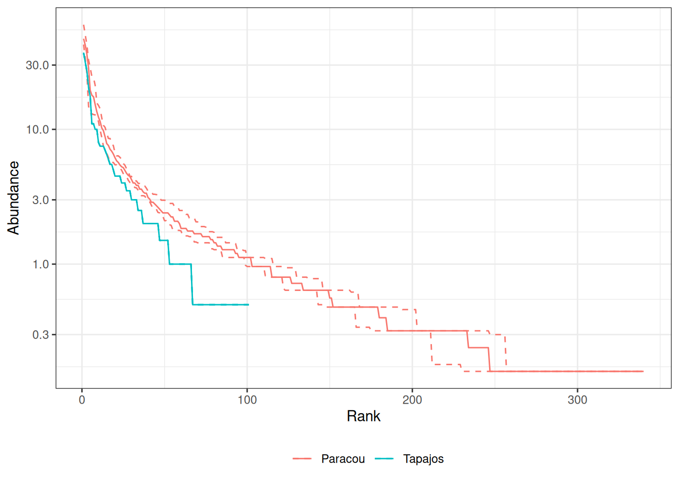
Species composition at the Paracou and Tapajos sites expressed in terms of species rank-abundance curve. Confidence intervals on inventory analysis at 95 % are shown with error bars and are based on among plots variations.