Structure v4

Calibration of forest structure parameters (crown radius allometry and mortality) in TROLL 4.0.1 (as mortality differs between TROLL 3.1.8 and 4.0.1):

\(m\) : minimal death rate in death per year calibrated with TROLL 3.1.8 to 0.055 both at Paracou and Tapajos
\(a_{CR}\) : crown radius intercept calibrated with TROLL 3.1.8 to 1.85 at Paracou and to 2.50 at Tapajos
\(b_{CR}\) : crown radius slope calibrated with TROLL 3.1.8 to 0.4445 at Paracou and to 0.8150 at Tapajos

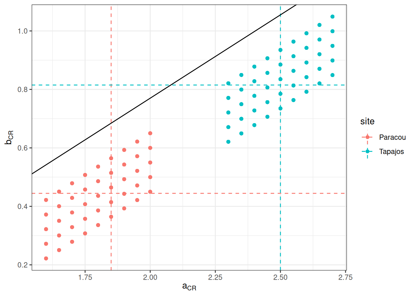
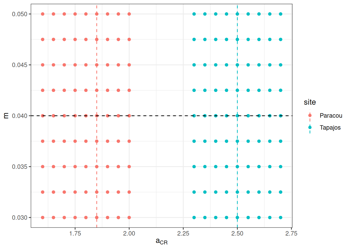
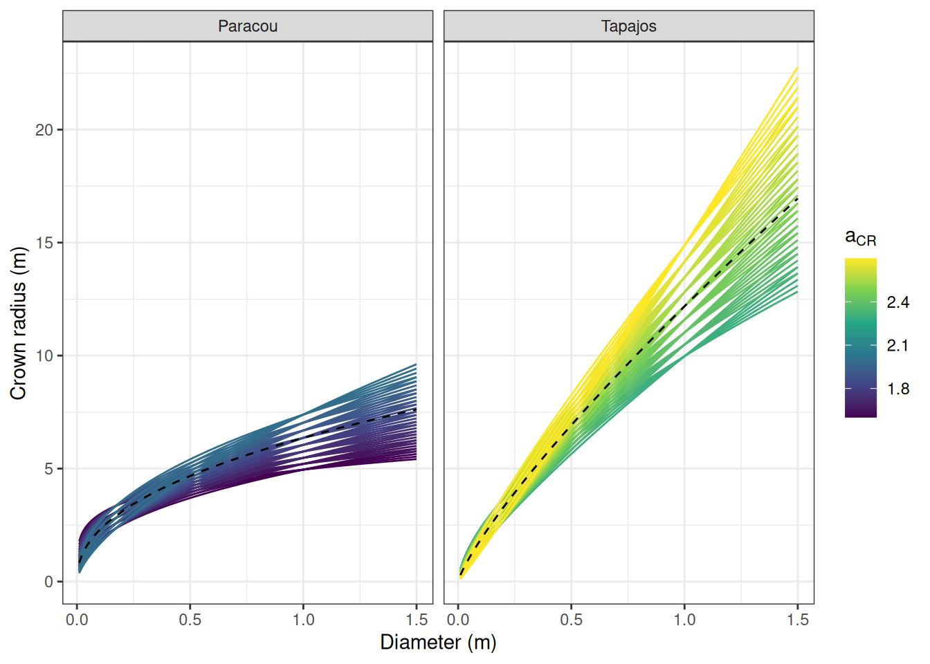
Parameters spaces

We prepared the parameter space for calibration defining low limit, high limit, and step for a, m, and the error of b for Paracou and Tapajos independently using calibration of forest crown radius allometry from TROLL 3.1.8 as prior and tests with TROLL 4.0.1 for the mortality prior. We obtained a calibration grid of 810 simulations. Dashed lines shows prior values. The last figure shows the corresponding projected allometries of crown radius.

Code

pars_par <- data.frame(site = "Paracou",
                       parameter = c("a", "error_b", "m"),
                       low = c(1.6, -6*0.05, 0.03),
                       high = c(2.0, -2*0.05, 0.05),
                       by = c(0.05, 0.05, 0.0025))
pars_tap <- data.frame(site = "Tapajos",
                       parameter = c("a", "error_b", "m"),
                       low = c(2.3, -6*0.05, 0.03),
                       high = c(2.7, -2*0.05, 0.05),
                       by = c(0.05, 0.05, 0.0025))
pars <- bind_rows(pars_par, pars_tap)
grid_par <- data.frame(a = seq(pars_par$low[1], pars_par$high[1], by = pars_par$by[1])) %>% 
  mutate(error_b = list(seq(pars_par$low[2], pars_par$high[2], by = pars_par$by[2]))) %>% 
  unnest(error_b) %>% 
  mutate(b = -0.39 + 0.57*a + error_b) %>% 
  mutate(m = list(seq(pars_par$low[3], pars_par$high[3], by = pars_par$by[3]))) %>% 
  unnest(m) %>% 
  mutate(site = "Paracou")
grid_tap <- data.frame(a = seq(pars_tap$low[1], pars_tap$high[1], by = pars_tap$by[1])) %>% 
  mutate(error_b = list(seq(pars_tap$low[2], pars_tap$high[2], by = pars_tap$by[2]))) %>% 
  unnest(error_b) %>% 
  mutate(b = -0.39 + 0.57*a + error_b) %>% 
  mutate(m = list(seq(pars_tap$low[3], pars_tap$high[3], by = pars_tap$by[3]))) %>% 
  unnest(m) %>% 
  mutate(site = "Tapajos")
grid <- bind_rows(grid_par, grid_tap)

Code

kable(pars)

site	parameter	low	high	by
Paracou	a	1.60	2.00	0.0500
Paracou	error_b	-0.30	-0.10	0.0500
Paracou	m	0.03	0.05	0.0025
Tapajos	a	2.30	2.70	0.0500
Tapajos	error_b	-0.30	-0.10	0.0500
Tapajos	m	0.03	0.05	0.0025

Code

grid %>% 
  ggplot(aes(a, b, col = site)) +
  geom_point() +
  geom_vline(aes(xintercept = a, col = site), linetype = "dashed", 
             data = data.frame(a = c(1.85, 2.50), site = c("Paracou", "Tapajos"))) +
  geom_hline(aes(yintercept = b, col = site), linetype = "dashed", 
             data = data.frame(b = c(0.4445, 0.8150), site = c("Paracou", "Tapajos"))) +
  geom_abline(intercept = -0.37, slope = 0.57, col = "black") +
  theme_bw() +
  xlab(expression(a[CR])) +
  ylab(expression(b[CR]))

Code

grid %>% 
  ggplot(aes(a, m, col = site)) +
  geom_point() +
  geom_vline(aes(xintercept = a, col = site), linetype = "dashed", 
             data = data.frame(a = c(1.85, 2.50), site = c("Paracou", "Tapajos"))) +
  geom_hline(yintercept = 0.040, linetype = "dashed") +
  theme_bw() +
  xlab(expression(a[CR])) +
  ylab(expression(m))

Code

grid %>% 
  mutate(dbh = list(seq(1, 150, 1)/100)) %>% 
  unnest(dbh) %>% 
  mutate(cr = exp(a+b*log(dbh))) %>% 
  ggplot(aes(dbh, cr)) +
  geom_line(aes(col = a, group = paste(a, b))) +
  theme_bw() +
  scale_colour_viridis_c(expression(a[CR])) +
  xlab("Diameter (m)") + ylab("Crown radius (m)") +
  geom_line(col = "black", linetype = "dashed",
            data = bind_rows(
              data.frame(site = "Paracou", 
                         dbh = seq(1, 150, 1)/100) %>% 
              mutate(cr = exp(1.85+0.4445*log(dbh))),
              data.frame(site = "Tapajos", 
                         dbh = seq(1, 150, 1)/100) %>% 
              mutate(cr = exp(2.50+0.8150*log(dbh)))
            )
              
            ) +
  facet_wrap(~ site)

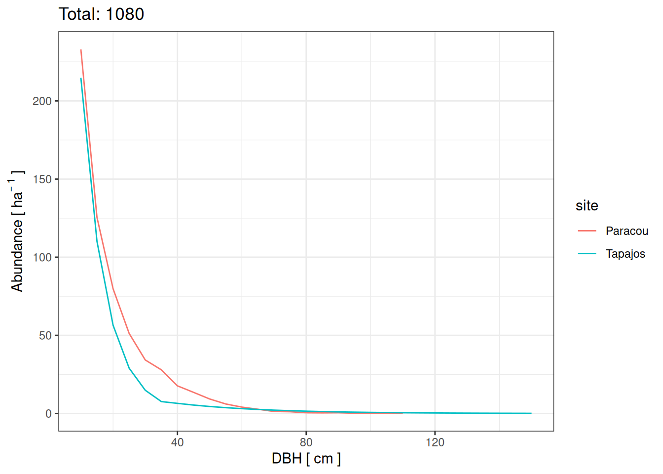
Observations

We used different evaluation metrics per site to rely on a single data source and minimise discrepancies.

For Tapajos and according to Rice et al. (2004) :

470 live trees per hectare with diameter at breast height (dbh) ≥10
Aboveground live biomass was 143.7 ± 5.4 Mg C/ha
Stem density -0.058 (±0.003) dbh_cm + 2.912 (±0.076) for dbh < 40
Stem density -0.016 (±0.001) dbh_cm + 1.451 (±0.04) for dbh > 40
Stem density is shown below

For Paracou according to the inventories:

612 ± 37 live trees per hectare with diameter at breast height (dbh) ≥10 (from inventory)
Basal area was 30.8 ± 0.836 m2/ha
Stem density is shown below

Code

abd_par <- read_tsv("outputs/inventories.tsv", show_col_types = FALSE) %>% 
  filter(site == "Paracou", type == "default") %>% 
  filter(dbh > 10) %>% 
  group_by(plot) %>% 
  summarise(abundance = n()/unique(plot_size)) %>% 
  ungroup()
# paste(round(median(abd_par$abundance)), "±", round(sd(abd_par$abundance)))
# read_tsv("outputs/inventories.tsv") %>% 
#   filter(site == "Paracou", type == "default", dbh >= 10) %>% 
#   group_by(plot) %>% 
#   summarise(ba = sum((dbh/2)^2*pi)/10^4/unique(plot_size)) %>% 
#   summarise(ba_mean = median(ba), ba_sd = sd(ba))
obs_tap <- data.frame(dbh_class = seq(10, 150, 5)) %>% 
  mutate(abundance = ifelse(dbh_class < 40, 
                            10^(-0.058*dbh_class+2.912), 
                            10^(-0.016*dbh_class+1.451))) %>% 
  mutate(site = "Tapajos")

obs_par <- read_tsv("outputs/inventories.tsv", show_col_types = FALSE) %>% 
  filter(site == "Paracou", type == "default") %>% 
  filter(dbh > 10) %>% 
  mutate(dbh_class = cut(dbh, 
                         breaks = c(seq(10, 155, by = 5)), 
                         labels = c(seq(10, 150, by = 5)))) %>% 
  mutate(dbh_class = as.numeric(as.character(dbh_class))) %>% 
    group_by(plot, dbh_class) %>% 
  summarise(abundance = n()/unique(plot_size)) %>% 
  group_by(dbh_class) %>% 
  summarise(abundance = median(abundance)) %>% 
  mutate(site = "Paracou")
# obs <- bind_rows(obs_tap, obs_par)
obs <- bind_rows(obs_tap, obs_par)
ggplot(obs, (aes(dbh_class, abundance, col = site))) +
  geom_line() +
  theme_bw() +
  xlab("DBH [ cm ]") + ylab(expression(Abundance~"["~ha^{-~1}~"]")) +
  ggtitle(paste("Total:", round(sum(obs$abundance))))

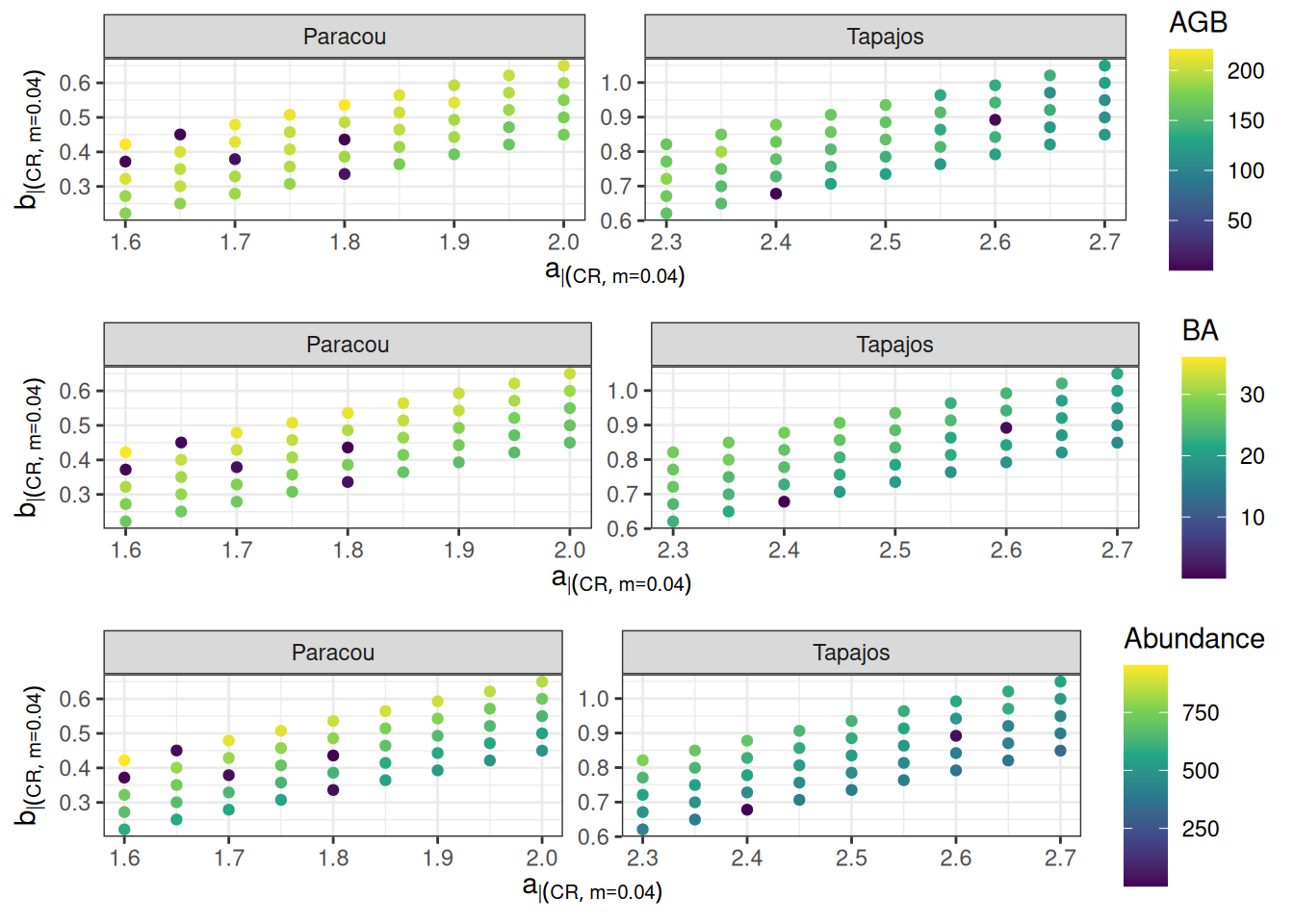
Parameters effect

Code

bind_rows(
  read_tsv("results/calib_str4_Paracou.tsv"),
  read_tsv("results/calib_str4_Tapajos.tsv")
) %>% 
  mutate(dbh_class = cut(dbh_cm, 
                         breaks = seq(10, 205, by = 5), 
                         labels = seq(10, 200, by = 5),
                         include.lowest = TRUE)) %>% 
  mutate(dbh_class = as.numeric(as.character(dbh_class))) %>% 
  group_by(site, a, b, m, dbh_class) %>% 
  summarise(abundance = n()/4, 
            agb = sum(agb)/4, 
            ba = sum((dbh_cm/2)^2*pi)/10^4/4) %>% 
  write_tsv("outputs/calib_str4.tsv")

\(a_{CR}\)

Code

dat <-  read_tsv("outputs/calib_str4.tsv") %>% 
  group_by(site, a, b, m) %>% 
  summarise(agb = sum(agb)/10^3/2,
            ba = sum(ba),
            abundance = sum(abundance)) %>% 
  filter(m == 0.040)
cowplot::plot_grid(
 dat %>% 
  ggplot(aes(a, b, col = agb)) +
  geom_point() +
  facet_wrap(~ site, scales = "free") +
  theme_bw() +
  scale_color_viridis_c("AGB") +
  xlab(expression(a[CR|m==0.04])) + ylab(expression(b[CR|m==0.04])),
  dat %>% 
  ggplot(aes(a, b, col = ba)) +
  geom_point() +
  facet_wrap(~ site, scales = "free") +
  theme_bw() +
  scale_color_viridis_c("BA") +
  xlab(expression(a[CR|m==0.04])) + ylab(expression(b[CR|m==0.04])),
   dat %>% 
  ggplot(aes(a, b, col = abundance)) +
  geom_point() +
  facet_wrap(~ site, scales = "free") +
  theme_bw() +
  scale_color_viridis_c("Abundance") +
  xlab(expression(a[CR|m==0.04])) + ylab(expression(b[CR|m==0.04])), 
 nrow = 3)

Code

read_tsv("outputs/calib_str4.tsv") %>% 
  group_by(site, a, b, m) %>% 
  summarise(abundance = sum(abundance), 
            agb = sum(agb)/10^3/2) %>% 
  ggplot(aes(abundance, agb, col = a)) +
  geom_point() +
  theme_bw() +
  scale_color_viridis_c(expression(a[CR])) +
  facet_wrap(~ site)

Code

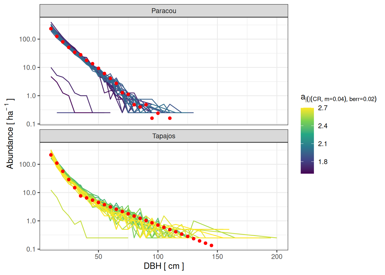
read_tsv("outputs/calib_str4.tsv") %>% 
  filter(m == 0.040) %>% 
  mutate(berr = -0.39 + 0.57*a - b) %>% 
  filter(berr > 0.1, berr < 0.3) %>% 
  ggplot(aes(dbh_class, abundance)) +
  geom_line(aes(col = a, group = paste(a, b, m))) +
  geom_point(data = filter(obs, dbh_class < 150), col = "red") +
  scale_y_log10(labels = scales::comma) +
  xlab("DBH [ cm ]") + ylab(expression(Abundance~"["~ha^{-~1}~"]")) +
  scale_color_viridis_c(expression(a[CR|m==0.04|berr==0.02])) +
  theme_bw() +
  facet_wrap(~ site, nrow = 2)

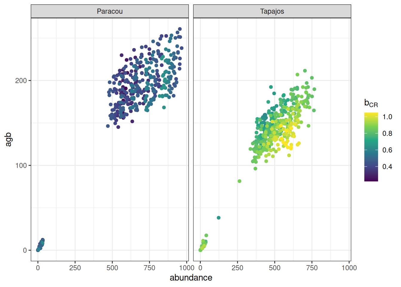
\(b_{CR}\)

Code

read_tsv("outputs/calib_str4.tsv") %>% 
  group_by(site, a, b, m) %>% 
  summarise(abundance = sum(abundance), 
            agb = sum(agb)/10^3/2) %>% 
  ggplot(aes(abundance, agb, col = b)) +
  geom_point() +
  theme_bw() +
  scale_color_viridis_c(expression(b[CR])) +
  facet_wrap(~ site)

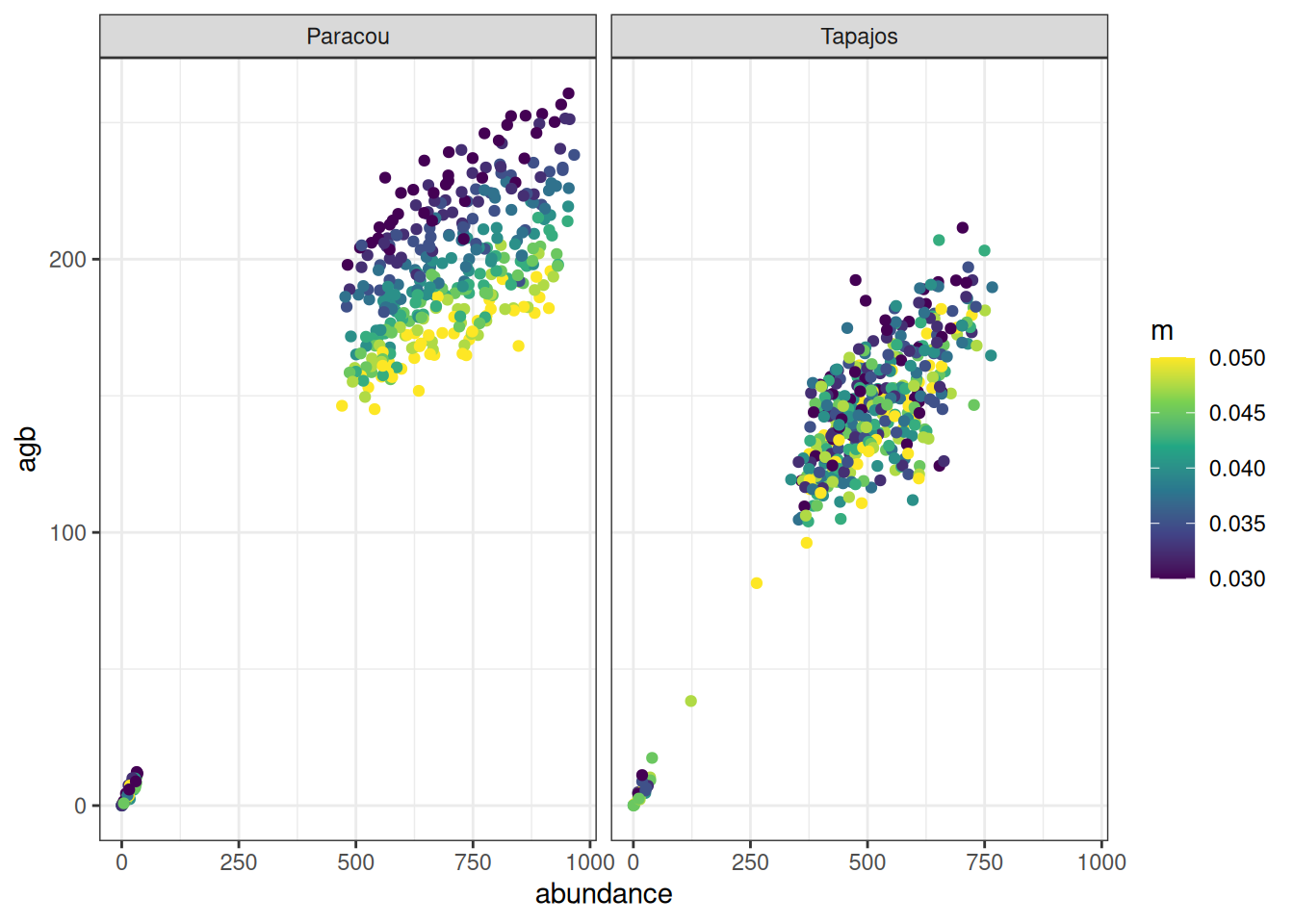
\(m\)

Code

read_tsv("outputs/calib_str4.tsv") %>% 
  group_by(site, a, b, m) %>% 
  summarise(abundance = sum(abundance), 
            agb = sum(agb)/10^3/2) %>% 
  ggplot(aes(abundance, agb, col = m)) +
  geom_point() +
  theme_bw() +
  scale_color_viridis_c(expression(m)) +
  facet_wrap(~ site)

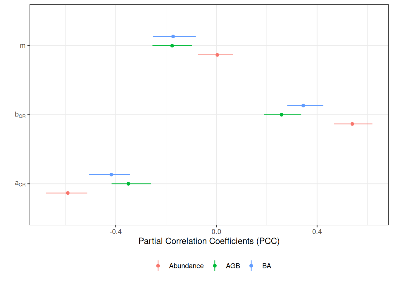
Sensitivity to parameters

Code

t <- read_tsv("outputs/calib_str4.tsv") %>% 
  group_by(site, a, b, m) %>% 
  summarise(abundance = sum(abundance), agb = sum(agb), ba = sum(ba))
sens <- lapply(c("abundance", "agb", "ba"), function(var) 
  sensitivity::pcc(t[c("a", "b", "m")], t[var], nboot = 100)$PCC %>%
                      rownames_to_column(var = "parameter") %>% 
    mutate(variable = var)) %>% 
  bind_rows()

Code

g <- sens %>% 
  mutate(parameter = recode(parameter,
                            "a" = "a[CR]",
                            "b" = "b[CR]",
                            "m" = "m")) %>% 
   mutate(variable = recode(variable,
                            "abundance" = "Abundance",
                            "agb" = "AGB",
                            "ba" = "BA")) %>% 
  ggplot(aes(parameter, original, col = variable)) + 
  geom_point(position = position_dodge(0.4)) + 
  theme_bw() +
  coord_flip() + 
  geom_linerange(aes(ymin = `min. c.i.`, ymax = `max. c.i.`), 
                 position = position_dodge(0.4)) + 
  ylab("Partial Correlation Coefficients (PCC)") + xlab("") +
  theme(legend.position = "bottom") +
  scale_x_discrete(labels = scales::label_parse()) +
  scale_colour_discrete("")
g

Best parameters

Paracou

Code

eval_par <- read_tsv("outputs/calib_str4.tsv") %>% 
  filter(site == "Paracou") %>% 
  select(site, a, b, m) %>% 
  unique() %>% 
  mutate(dbh_class = list(seq(10, 150, by = 5))) %>% 
  unnest(dbh_class) %>% 
  left_join(read_tsv("outputs/calib_str4.tsv")) %>% 
  select(-agb) %>% 
  mutate_at(c("abundance", "ba"), ~ifelse(is.na(.), 0, .)) %>% 
  rename(simulated = abundance) %>% 
  left_join(rename(obs, observed = abundance)) %>% 
  mutate(observed = ifelse(is.na(observed), 0, observed)) %>% 
  group_by(site, a, b, m) %>% 
  summarise(rmsep_dist = sqrt(mean((observed - simulated)^2)),
            rmsep_ba = sqrt((30.8 - sum(ba))^2),
            rmsep_abund = sqrt((612 - sum(simulated))^2)
            ) %>% 
  ungroup() %>% 
  mutate(all_rmsep_norm = rmsep_dist/30.5 + rmsep_ba/30.8 + rmsep_abund/612) %>% 
  mutate(sim = paste0(site, "_", a, "_", b, "_", m))
best_par <- eval_par %>% 
  group_by(site) %>% 
  slice_min(all_rmsep_norm, n = 5)

Code

read_tsv("outputs/calib_str4.tsv") %>% 
  mutate(sim = paste0(site, "_", a, "_", b, "_", m)) %>% 
  left_join(best_par) %>% 
  filter(!is.na(all_rmsep_norm)) %>% 
  group_by(site, a, b, m) %>% 
  summarise(abundance = sum(abundance), ba = sum(ba)) %>% 
  gather(variable, value, -site) %>% 
  group_by(site, variable) %>% 
  summarise(median = median(value), minimum = min(value), maximum = max(value)) %>% 
  knitr::kable(caption = "Best structure parameters according to calibration with inventory data.")

Best structure parameters according to calibration with inventory data.
site	variable	median	minimum	maximum
Paracou	a	1.8000	1.80000	1.90000
Paracou	abundance	606.2500	587.50000	628.00000
Paracou	b	0.3860	0.38600	0.44300
Paracou	ba	30.0482	29.46175	32.09072
Paracou	m	0.0325	0.03250	0.03750

Code

read_tsv("outputs/calib_str4.tsv") %>% 
  mutate(sim = paste0(site, "_", a, "_", b, "_", m)) %>% 
  left_join(best_par %>% slice_min(all_rmsep_norm)) %>% 
  filter(!is.na(all_rmsep_norm)) %>% 
  ggplot(aes(dbh_class, abundance)) +
  geom_line(aes(group = sim)) +
  geom_point(data = obs %>% filter(site == "Paracou"), col = "red") +
  scale_y_log10(labels = scales::comma) +
  xlab("DBH [ cm ]") + ylab(expression(Abundance~"["~ha^{-~1}~"]")) +
  theme_bw() +
  facet_wrap(~ site)

Tapajos

Code

eval_tap <- read_tsv("outputs/calib_str4.tsv") %>% 
  filter(site == "Tapajos") %>% 
  select(site, a, b, m) %>% 
  unique() %>% 
  mutate(dbh_class = list(seq(10, 150, by = 5))) %>% 
  unnest(dbh_class) %>% 
  left_join(read_tsv("outputs/calib_str4.tsv")) %>% 
  select(-ba) %>% 
  mutate_at(c("abundance", "agb"), ~ifelse(is.na(.), 0, .)) %>% 
  rename(simulated = abundance) %>% 
  left_join(rename(obs, observed = abundance)) %>% 
  mutate(observed = ifelse(is.na(observed), 0, observed)) %>% 
  group_by(site, a, b, m) %>% 
  summarise(rmsep_dist = sqrt(mean((observed - simulated)^2)),
            rmsep_agb = sqrt((143.7 - sum(agb)/10^3/2)^2),
            rmsep_abund = sqrt((470 - sum(simulated))^2)
            ) %>% 
  ungroup() %>% 
  mutate(all_rmsep_norm = rmsep_dist/16.2 + rmsep_agb/143.7 + rmsep_abund/470) %>% 
  mutate(sim = paste0(site, "_", a, "_", b, "_", m))
best_tap <- eval_tap %>% 
  group_by(site) %>% 
  slice_min(all_rmsep_norm, n = 5)

Code

read_tsv("outputs/calib_str4.tsv") %>% 
  mutate(sim = paste0(site, "_", a, "_", b, "_", m)) %>% 
  left_join(best_tap) %>% 
  filter(!is.na(all_rmsep_norm)) %>% 
  group_by(site, a, b, m) %>% 
  summarise(abundance = sum(abundance), agb = sum(agb)/10^3/2) %>% 
  gather(variable, value, -site) %>% 
  group_by(site, variable) %>% 
  summarise(median = median(value), minimum = min(value), maximum = max(value)) %>% 
  knitr::kable(caption = "Best structure parameters according to calibration with inventory data.")

Best structure parameters according to calibration with inventory data.
site	variable	median	minimum	maximum
Tapajos	a	2.4500	2.3500	2.5000
Tapajos	abundance	467.0000	460.2500	484.2500
Tapajos	agb	144.8843	139.7424	148.6621
Tapajos	b	0.7565	0.6995	0.7850
Tapajos	m	0.0400	0.0300	0.0500

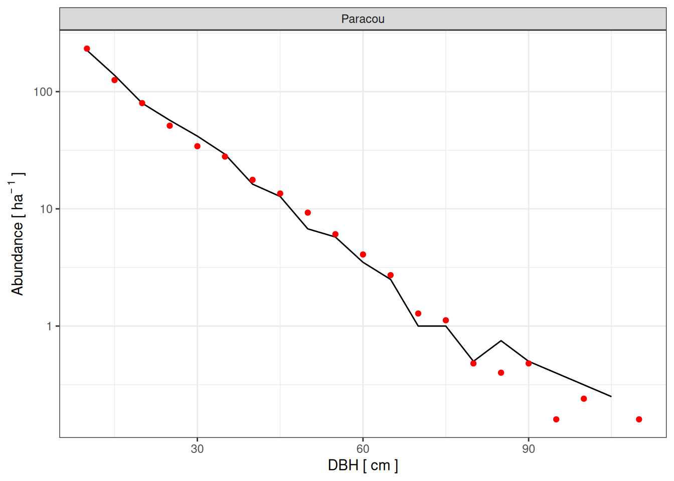
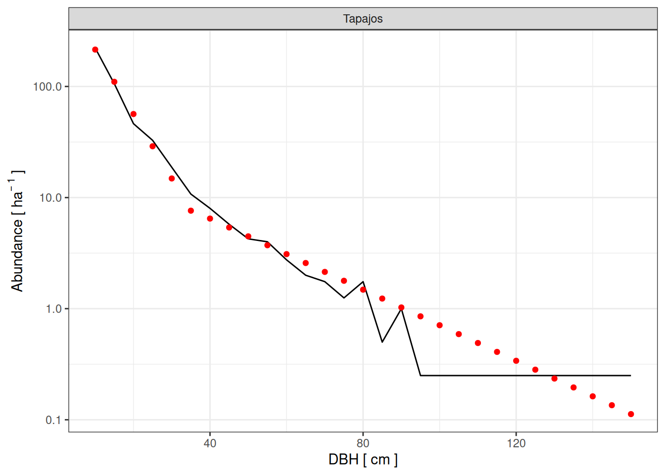
Code

read_tsv("outputs/calib_str4.tsv") %>% 
  mutate(sim = paste0(site, "_", a, "_", b, "_", m)) %>% 
  left_join(best_tap %>% slice_min(all_rmsep_norm)) %>% 
  filter(!is.na(all_rmsep_norm)) %>% 
  ggplot(aes(dbh_class, abundance)) +
  geom_line(aes(group = sim)) +
  geom_point(data = obs %>% filter(site == "Tapajos"), col = "red") +
  scale_y_log10(labels = scales::comma) +
  xlab("DBH [ cm ]") + ylab(expression(Abundance~"["~ha^{-~1}~"]")) +
  theme_bw() +
  facet_wrap(~ site)

All

Code

read_tsv("outputs/calib_str4.tsv") %>% 
  select(site, a, b, m) %>% 
  unique() %>% 
  mutate(dbh_class = list(seq(10, 150, by = 5))) %>% 
  unnest(dbh_class) %>% 
  left_join(read_tsv("outputs/calib_str4.tsv")) %>% 
  select(-agb, -ba) %>% 
  mutate(abundance = ifelse(is.na(abundance), 0, abundance)) %>% 
  rename(simulated = abundance) %>% 
  left_join(rename(obs, observed = abundance)) %>% 
  mutate(observed = ifelse(is.na(observed), 0, observed)) %>% 
  group_by(site, a, b, m) %>% 
  summarise(normal = sqrt(mean((observed - simulated)^2)),
            lognormal = exp(sqrt(mean((log(observed+1) - log(simulated+1))^2)))) %>% 
  gather(metric, rmsep, -site, -a, -b, -m) %>% 
  group_by(site, metric) %>% 
  slice_min(rmsep, n = 5) %>% 
  mutate(rmsep = round(rmsep, 2)) %>% 
  summarise(
    RMSEP = paste0(median(rmsep), " [", min(rmsep), "-", max(rmsep), "]"),
    a = paste0(median(a), " [", min(a), "-", max(a), "]"),
    b = paste0(median(b), " [", min(b), "-", max(b), "]"),
    m = paste0(median(m), " [", min(m), "-", max(m), "]")
  ) %>% 
  knitr::kable()

Rows: 15261 Columns: 8
── Column specification ────────────────────────────────────────────────────────
Delimiter: "\t"
chr (1): site
dbl (7): a, b, m, dbh_class, abundance, agb, ba

ℹ Use `spec()` to retrieve the full column specification for this data.
ℹ Specify the column types or set `show_col_types = FALSE` to quiet this message.
Rows: 15261 Columns: 8
── Column specification ────────────────────────────────────────────────────────
Delimiter: "\t"
chr (1): site
dbl (7): a, b, m, dbh_class, abundance, agb, ba

ℹ Use `spec()` to retrieve the full column specification for this data.
ℹ Specify the column types or set `show_col_types = FALSE` to quiet this message.
Joining with `by = join_by(site, a, b, m, dbh_class)`
Joining with `by = join_by(site, dbh_class)`
`summarise()` has grouped output by 'site', 'a', 'b'. You can override using the `.groups` argument.
`summarise()` has grouped output by 'site'. You can override using the `.groups` argument.

site	metric	RMSEP	a	b	m
Paracou	lognormal	1.12 [1.11-1.14]	1.8 [1.65-2]	0.386 [0.3005-0.55]	0.0325 [0.0325-0.035]
Paracou	normal	2.4 [1.38-2.7]	1.85 [1.8-1.9]	0.4145 [0.386-0.443]	0.0425 [0.0325-0.05]
Tapajos	lognormal	1.22 [1.19-1.22]	2.55 [2.5-2.7]	0.9135 [0.8635-0.9635]	0.0325 [0.03-0.045]
Tapajos	normal	2.54 [2.38-2.74]	2.35 [2.3-2.35]	0.6995 [0.671-0.6995]	0.045 [0.0375-0.05]

Code

bind_rows(
  eval_par %>% 
  select(-sim) %>% 
  gather(metric, rmsep, -site, -a, -b, -m) %>% 
  mutate(metric = gsub("rmsep_", "", metric)),
  eval_tap %>% 
  select(-sim) %>% 
  gather(metric, rmsep, -site, -a, -b, -m) %>% 
  mutate(metric = gsub("rmsep_", "", metric))
) %>% 
  group_by(site, metric) %>% 
  slice_min(rmsep, n = 5) %>% 
  mutate(rmsep = round(rmsep, 2)) %>% 
  summarise(
    RMSEP = paste0(median(rmsep), " [", min(rmsep), "-", max(rmsep), "]"),
    a = paste0(median(a), " [", min(a), "-", max(a), "]"),
    b = paste0(median(b), " [", min(b), "-", max(b), "]"),
    m = paste0(median(m), " [", min(m), "-", max(m), "]")
  ) %>% 
  write_tsv("figures/table_a4.tsv")
read_tsv("figures/table_a4.tsv") %>% 
  knitr::kable()

site	metric	RMSEP	a	b	m
Paracou	abund	5.75 [2-7.75]	1.75 [1.75-1.8]	0.3575 [0.3575-0.386]	0.0475 [0.0375-0.05]
Paracou	all_norm	0.16 [0.13-0.17]	1.8 [1.8-1.9]	0.386 [0.386-0.443]	0.0325 [0.0325-0.0375]
Paracou	ba	0.04 [0.03-0.07]	1.85 [1.65-2]	0.4715 [0.3505-0.5075]	0.0325 [0.03-0.05]
Paracou	dist	2.4 [1.38-2.7]	1.85 [1.8-1.9]	0.4145 [0.386-0.443]	0.0425 [0.0325-0.05]
Tapajos	abund	3 [0-3.5]	2.5 [2.4-2.65]	0.785 [0.728-0.9205]	0.035 [0.03-0.04]
Tapajos	agb	0.13 [0.04-0.19]	2.45 [2.35-2.5]	0.835 [0.6495-0.885]	0.045 [0.03-0.05]
Tapajos	all_norm	0.25 [0.18-0.25]	2.45 [2.35-2.5]	0.7565 [0.6995-0.785]	0.04 [0.03-0.05]
Tapajos	dist	2.54 [2.38-2.74]	2.35 [2.3-2.35]	0.6995 [0.671-0.6995]	0.045 [0.0375-0.05]

Code

bind_rows(
  best_par %>% slice_min(all_rmsep_norm),
  best_tap %>% slice_min(all_rmsep_norm)
) %>% 
  select(site, a, b, m) %>% 
  mutate(berr = b + 0.39 - 0.57*a) %>% 
  kable()

site	a	b	m	berr
Paracou	1.80	0.3860	0.035	-0.25
Tapajos	2.45	0.7565	0.040	-0.25

Code

bind_rows(best_par, best_tap) %>% 
  select(site, all_rmsep_norm, a, b, m) %>% 
  gather(parameter, value, -site, -all_rmsep_norm) %>% 
  group_by(site, parameter) %>% 
  arrange(all_rmsep_norm) %>% 
  summarise(minimum = min(value), median = median(value), 
            best = first(value), maximum = max(value)) %>% 
  kable()

site	parameter	minimum	median	best	maximum
Paracou	a	1.8000	1.8000	1.8000	1.9000
Paracou	b	0.3860	0.3860	0.3860	0.4430
Paracou	m	0.0325	0.0325	0.0350	0.0375
Tapajos	a	2.3500	2.4500	2.4500	2.5000
Tapajos	b	0.6995	0.7565	0.7565	0.7850
Tapajos	m	0.0300	0.0400	0.0400	0.0500

Code

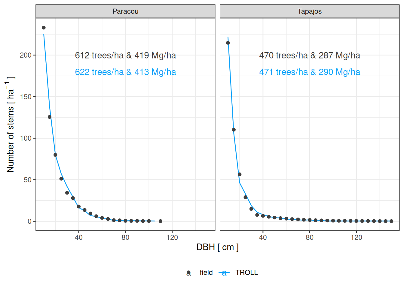
g <- read_tsv("outputs/calib_str4.tsv") %>% 
  mutate(sim = paste0(site, "_", a, "_", b, "_", m)) %>% 
  left_join(
    bind_rows(
      best_tap %>% slice_min(all_rmsep_norm),
      best_par %>% slice_min(all_rmsep_norm)
    )
  ) %>% 
  filter(!is.na(all_rmsep_norm)) %>% 
  ggplot(aes(dbh_class, abundance)) +
  geom_line(aes(group = sim, col = "TROLL")) +
  geom_point(data = obs, aes(col = "field")) +
  xlab("DBH [ cm ]") + ylab(expression(Number~of~stems~"["~ha^{-~1}~"]")) +
  theme_bw() +
  facet_wrap(~ site) +
  scale_colour_manual("", values = c("#3f3f3f", "#0da1f8")) +
  theme(legend.position = "bottom") +
  geom_text(aes(col = "field", label = lab), 
            data = data.frame(dbh_class = 80, abundance = 200,
                              lab = c("470 trees/ha & 287 Mg/ha",
                                      "612 trees/ha & 419 Mg/ha"),
                              site = c("Tapajos", "Paracou"))) +
  geom_text(aes(col = "TROLL", label = lab), 
            data = data.frame(dbh_class = 80, abundance = 180,
                              lab = c("471 trees/ha & 290 Mg/ha",
                                      "622 trees/ha & 413 Mg/ha"),
                              site = c("Tapajos", "Paracou")))
ggsave("figures/f01.png", g, dpi = 300, width = 8, height = 5, bg = "white")
g

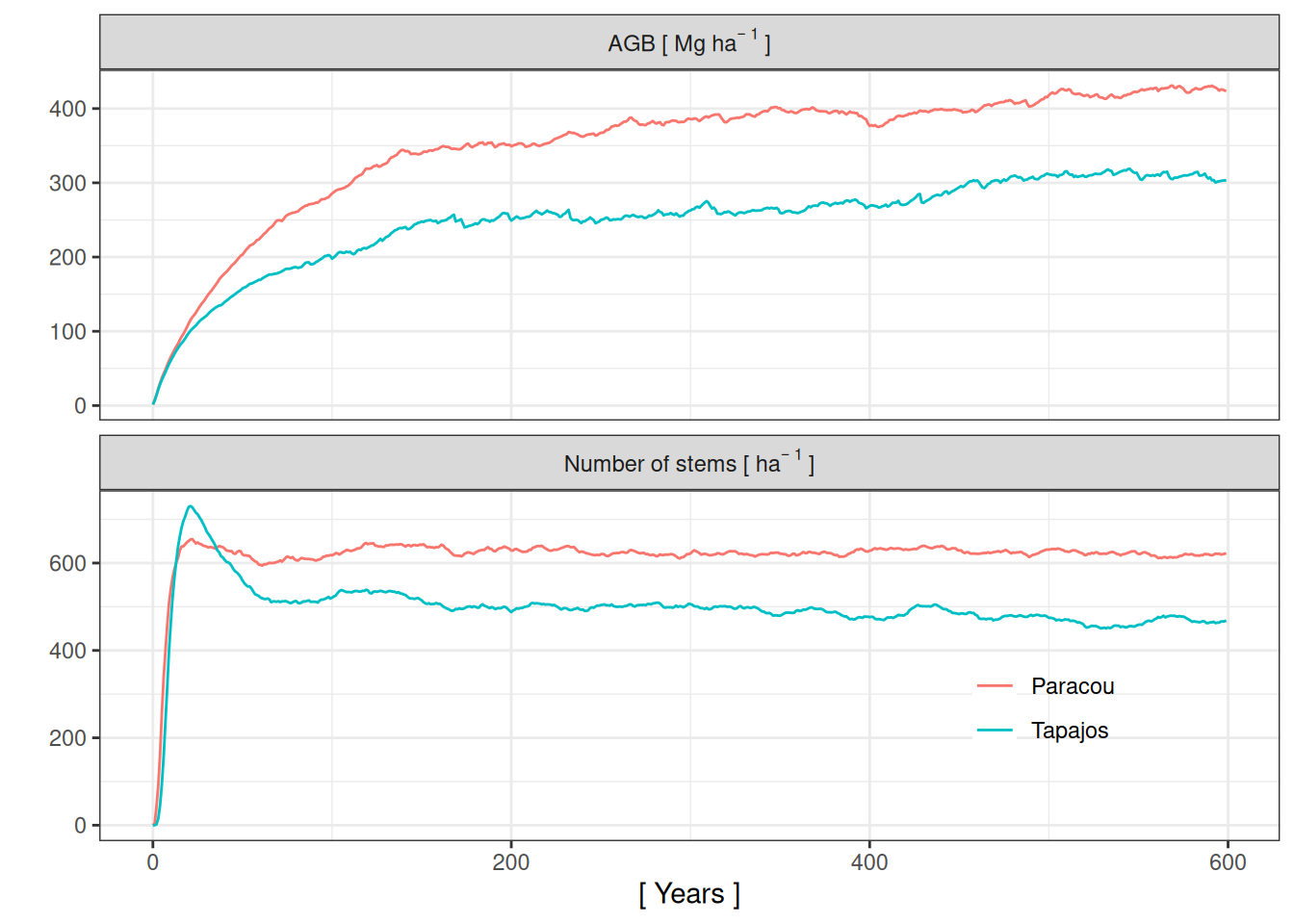
Spinup

Code

spinup <- list(
  Paracou = read_tsv("results/calib_str4_run/Paracou_1.8_-0.25_0.035/Paracou_1.8_-0.25_0.035_0_sumstats.txt") %>% 
    mutate(date = as_date("0000/01/01")+iter),
  Tapajos = read_tsv("results/calib_str4_run/Tapajos_2.45_-0.25_0.04/Tapajos_2.45_-0.25_0.04_0_sumstats.txt") %>% 
    mutate(date = as_date("0000/01/01")+iter)
) %>% 
  bind_rows(.id = "site") %>% 
  group_by(site, year = year(date)) %>% 
  summarise(abundance = mean(sum10), agb = mean(agb)/10^3) %>% 
  gather(variable, value, -year, -site)
g <- spinup %>% 
  mutate(var_long = recode(variable, 
                           "agb" = 'AGB~"["~Mg~ha^{-~1}~"]"',
                           "abundance" = 'Number~of~stems~"["~ha^{-~1}~"]"')) %>% 
  ggplot(aes(year, value, col = site)) + 
   geom_line() + 
   facet_wrap(~ var_long, scales = "free_y", nrow = 3, labeller = label_parsed) + 
   theme_bw() +
  xlab("[ Years ]") + ylab("") + scale_colour_discrete("") +
  theme(legend.position = c(0.8, 0.2), legend.background = element_blank())
ggsave("figures/fa03.png", g, dpi = 300, width = 10, height = 5, bg = "white")
g