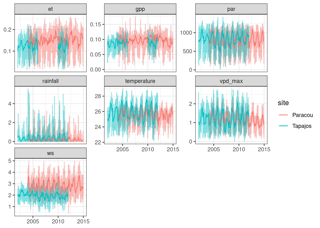
Climatic data for Paracou and Tapajos used to calibrate the new leaf phenology module in TROLL version 4 and evaluate simulation results.
Carbon and water fluxes - FLUXNET
FLUXNET 2015 (Pastorello, Gilberto et al. 2020) at Paracou and Tapajos was retrieved freely from FLUXNET (the manifest is available in data). They are mainly used for TROLL model forcing but also include fluxes for TROLL simulations validation including growth primary productivity (GPP) and evapotranspiration (ET). We also computed Photosynthetically Active Radiation (PAR) as it is a driver of GPP, and daily maximum Vapour Pressure Deficit (VPD) as it is a driver of ET. We removed GPP and ET data between 2006 and 2009 in Tapajos due to a known incident with the sensors.
The FLUXNET2015 Dataset includes data collected at sites from multiple regional flux networks. The preparation of this FLUXNET Dataset has been possible thanks only to the efforts of many scientists and technicians around the world and the coordination among teams from regional networks.
PI: Damien Bonal (Paracou), Mike Goulden (Tapajos), Scott Saleska (Tapajos)
Code
lambda <-function(t_air) 2.501- (2.361*10^-3)*t_airfluxnet <-list("Paracou"="data/climate/FLX_GF-Guy_FLUXNET2015_SUBSET_HH_2004-2014_2-4.csv","Tapajos"="data/climate/FLX_BR-Sa1_FLUXNET2015_SUBSET_HR_2002-2011_1-4.csv") %>%lapply(vroom::vroom, na ="-9999") %>%bind_rows(.id ="site") %>%select(site, TIMESTAMP_START, TIMESTAMP_END, P_F, SW_IN_F, TA_F, VPD_F, WS_F, GPP_NT_VUT_REF, LE_F_MDS) %>%mutate(time =as_datetime(as.character(as.POSIXlt(as.character(TIMESTAMP_START), format ="%Y%m%d%H%M")))) %>%rename(rainfall = P_F, snet = SW_IN_F, temperature = TA_F, vpd = VPD_F, ws = WS_F,gpp = GPP_NT_VUT_REF, le = LE_F_MDS) %>%mutate(et =10^-6*le*60*30/lambda(temperature)) %>%# W.m-2.half-hour to MJ.s-1 to kg.m-2.half-hourmutate(et =ifelse(hour(time) %in%7:18, et, NA)) %>%mutate(vpd = vpd/10,gpp = gpp/100, par = snet*2.27*60*30/10^3) %>%select(site, time, vpd, par, gpp, et, rainfall, ws,temperature)fluxnet_tapajos <-filter(fluxnet, site =="Tapajos")era <- vroom::vroom("data/climate/era5_tapajos.csv") %>%filter(year(date) >2001) %>%mutate(time =as_datetime(date), rainfall = precipitation) %>%select(time, rainfall)fluxnet_tapajos <- fluxnet_tapajos %>%select(-rainfall) %>%left_join(era)time_freq <-0.5# TROLL v4start <-as_datetime(as_date(min(fluxnet_tapajos$time))) # to start from 00:30stop <-max(fluxnet_tapajos$time) +30*60# to stop at 23:00time <-seq(start, stop, by =60*60* time_freq)data <-left_join(tibble(time = time), fluxnet_tapajos,by ="time" ) %>%group_by(date =as_date(time)) %>%mutate(across(c(temperature, vpd, ws, gpp),~ zoo::na.spline(., time, na.rm =FALSE))) %>%mutate(across(c(par, et),~ zoo::na.approx(., time, na.rm =FALSE))) %>%ungroup() %>%select(-date) %>%mutate(across(c(par), ~ifelse(is.na(.), 0, .))) %>%mutate(across(c(par), ~ifelse(. <0, 0, .))) %>%mutate(site ="Tapajos")bind_rows(filter(fluxnet, site =="Paracou"), data) %>%mutate(vpd_max = vpd) %>%select(-vpd) %>%gather(variable, value, -site, -time) %>%group_by(site, variable, date =date(time)) %>%select(-time) %>%mutate(value =ifelse(value %in%c("et", "par", "rainfall"),sum(value, na.rm = T), value)) %>%mutate(value =ifelse(variable %in%c("vpd_max"),max(value, na.rm = T), value)) %>%summarise_all(mean, na.rm = T) %>%mutate(value =ifelse(variable %in%c("et", "gpp") & site =="Tapajos"&year(date) %in%2006:2009,NA, value)) %>%write_tsv("outputs/fluxnet_fluxes.tsv")
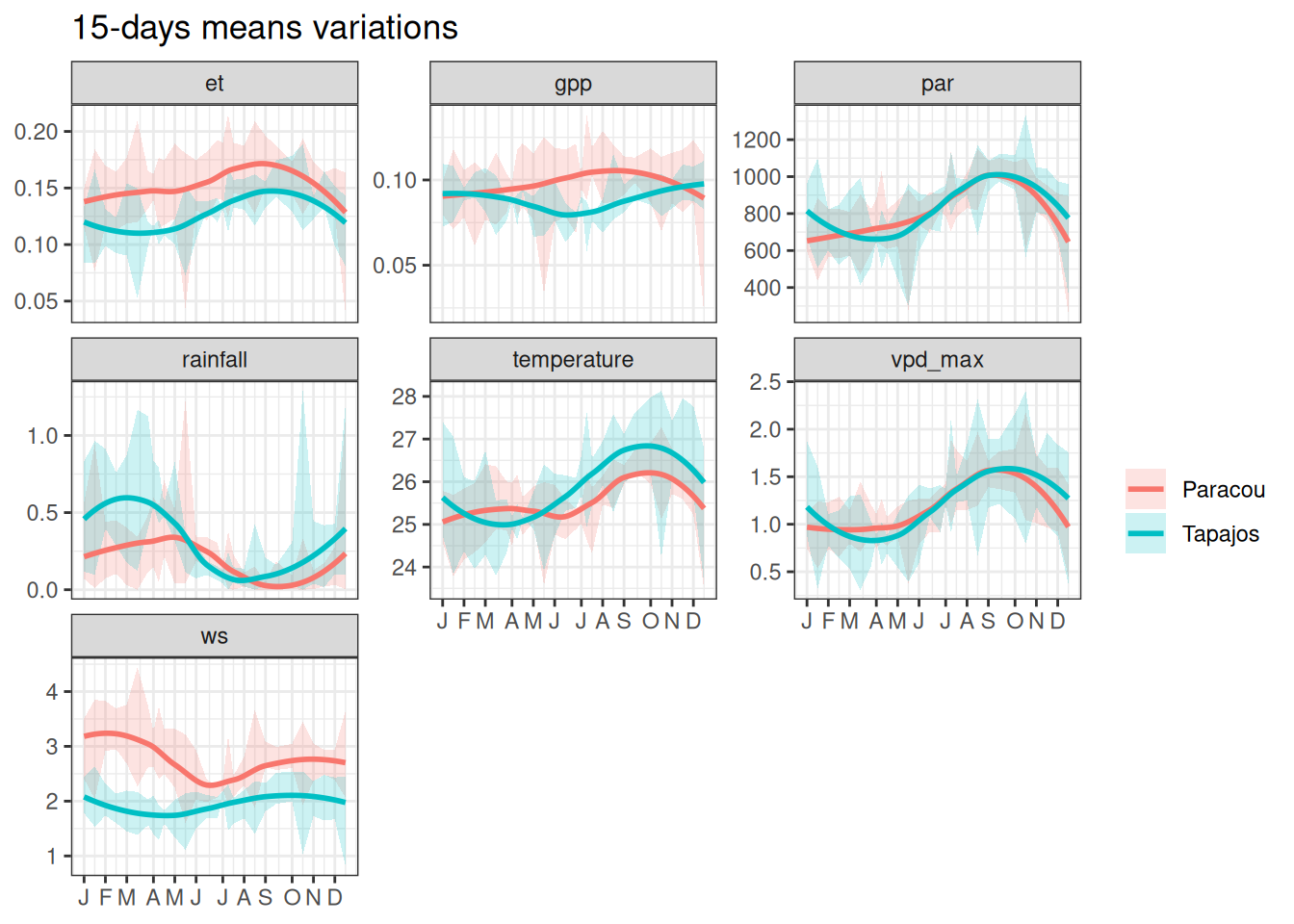
Mean annual cycle of fortnightly means of fluxes at Paracou and Tapajos across ten years.
Code
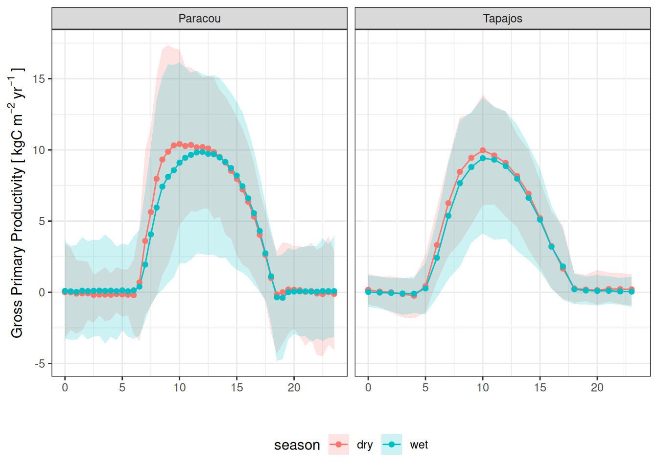
list("Paracou"="data/climate/FLX_GF-Guy_FLUXNET2015_SUBSET_HH_2004-2014_2-4.csv","Tapajos"="data/climate/FLX_BR-Sa1_FLUXNET2015_SUBSET_HR_2002-2011_1-4.csv") %>%lapply(vroom::vroom, na ="-9999") %>%bind_rows(.id ="site") %>%select(site, TIMESTAMP_START, TIMESTAMP_END, P_F, SW_IN_F, TA_F, VPD_F, WS_F, GPP_NT_VUT_REF, LE_F_MDS) %>%mutate(time =as_datetime(as.character(as.POSIXlt(as.character(TIMESTAMP_START), format ="%Y%m%d%H%M")))) %>%rename(gpp = GPP_NT_VUT_REF) %>%mutate(gpp = gpp/100*10^2*365/10^3) %>%select(site, time, gpp) %>%mutate(d_start =ifelse(site =="Paracou", yday("2020/08/01"), yday("2020/06/15"))) %>%mutate(d_end =ifelse(site =="Paracou", yday("2020/12/01"), yday("2020/11/01"))) %>%mutate(season =ifelse(yday(time) %in% d_start:d_end, "dry", "wet")) %>%group_by(site, season, time = hms::as_hms(time)) %>%summarise(l =quantile(gpp, 0.025, na.rm =TRUE), m =mean(gpp, na.rm =TRUE), h =quantile(gpp, 0.975, na.rm =TRUE)) %>%mutate(time =as.numeric(time)/(60*60)) %>%ggplot(aes(time, m, col = season, fill = season)) +geom_ribbon(aes(ymin = l, ymax = h), col =NA, alpha =0.2) +geom_line() +geom_point() +theme_bw() +facet_wrap(~ site) +theme(legend.position ="bottom") +ylab(expression("Gross Primary Productivity ["~kgC~m^{-2}~yr^{-1}~"]")) +xlab("")
GPP half-hourly.
Carbon flux - TROPOMI SIF
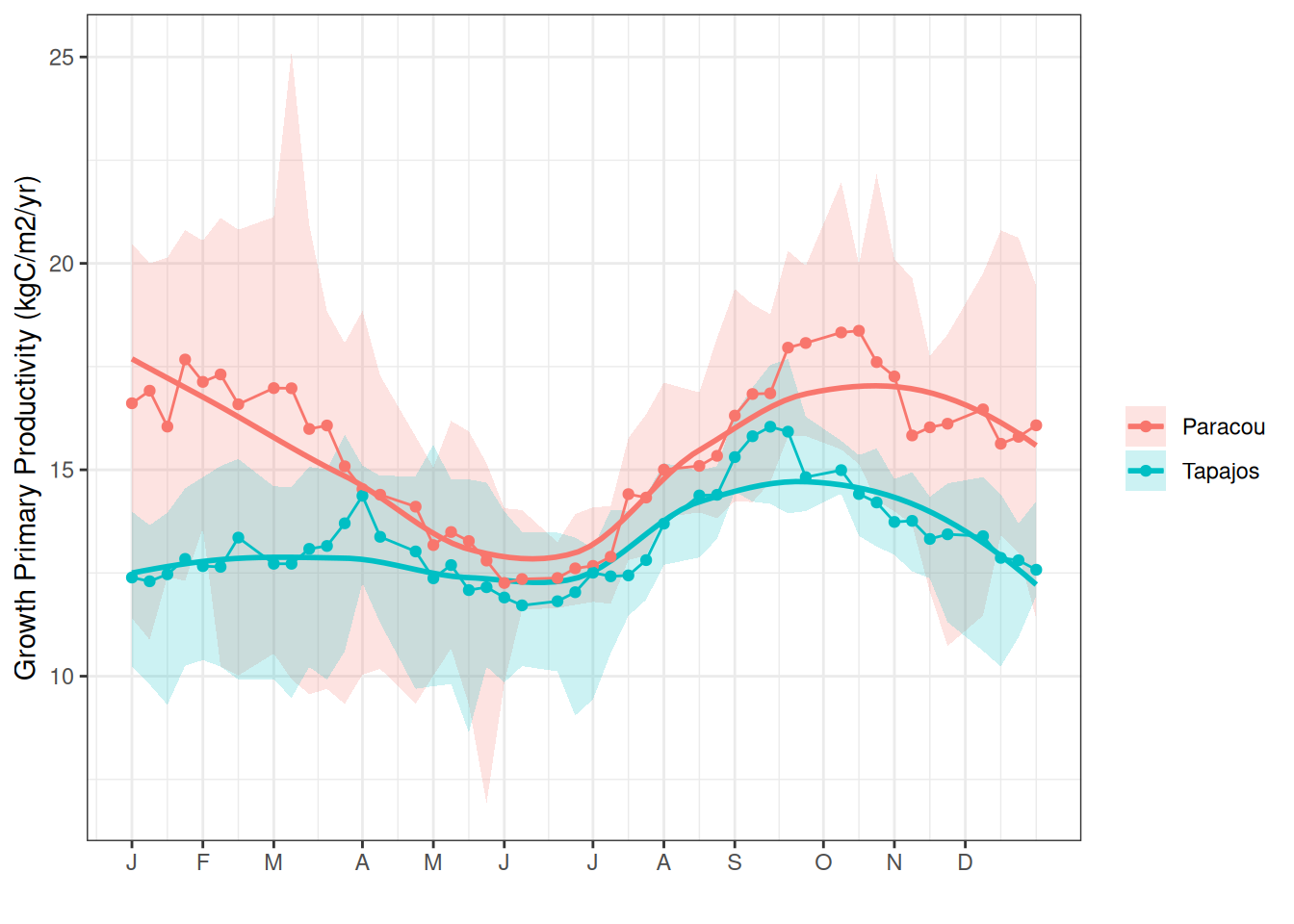
Tapajos and Paracou Solar Induced Fluorescence (SIF) from TROPOMI satellites was retrieved from https://figshare.com/ndownloader/articles/19336346/versions/2 and processed with the R script available in data. The SIF values were converted in Growth Primary Productivity (GPP) using \(GPP = 15.343 \times SIF\) following Chen et al. (2022).
Mean annual cycle of 8-days GPP derived from TROPOMI SIF at Paracou and Tapajos across ten years.
Soil water content
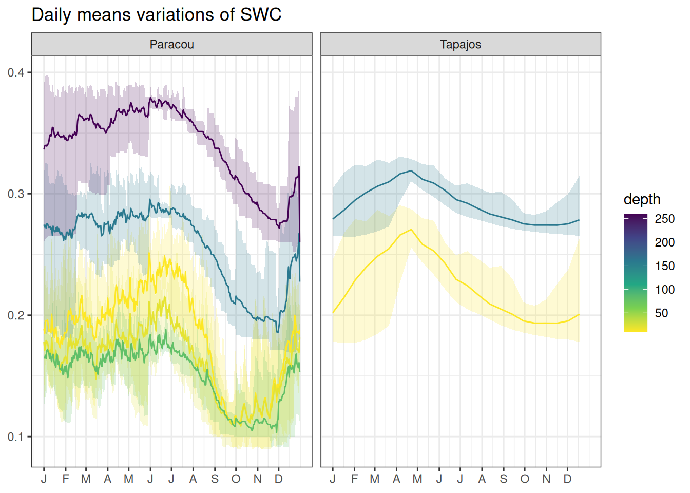
Guyaflux are Paracou Eddy Flux tower raw data (BONAL et al. 2008) from 2004 to 2022. Vapour Pressure Deficit (VPD, kPa) is computed from relative humidity (%). Data are available on demand and can be partly retrieved from PLUMBER2 (Ukkola, Abramowitz, and De Kauwe 2022) or FLUXNET (Pastorello, Gilberto et al. 2020). Guyaflux was mainly used for TROLL simulations validation including soil water content (SWC) at different depths. TROLL 4.0 water fluxes were assessed using the relative variation of soil water content (RSWC, %) from the top horizon from Paracou eddy flux tower (Bonal et al., 2008) and from reanalysed top horizon eddy flux tower against climatic water deficit at Tapajos (Restrepo-Coupe et al., 2024), defined as the daily mean value of soil water content (m3.m-3) divided by the yearly 95th quantile of daily mean.
read_tsv("outputs/guyaflux_swc.tsv") %>%mutate(depth =as.numeric(gsub("swc", "", variable))) %>%group_by(site, depth, day =yday(date)) %>%summarise(l =quantile(value, 0.025, na.rm =TRUE), m =mean(value, na.rm =TRUE), h =quantile(value, 0.975, na.rm =TRUE)) %>%ggplot(aes(day, m, col = depth, fill = depth, group = depth)) +geom_ribbon(aes(ymin = l, ymax = h), col =NA, alpha =0.2) +geom_line() +theme_bw() +scale_color_viridis_c(direction =-1) +scale_fill_viridis_c(direction =-1) +theme(axis.title =element_blank()) +facet_wrap(~ site) +ggtitle("Daily means variations of SWC") +scale_x_continuous(breaks =c(1, 32, 61, 92, 122, 153, 183, 214, 245, 275, 306, 336),labels =c("J", "F", "M", "A", "M", "J", "J", "A", "S", "O", "N", "D"))
Mean annual cycle of daily means of soil water content.
Litterfall
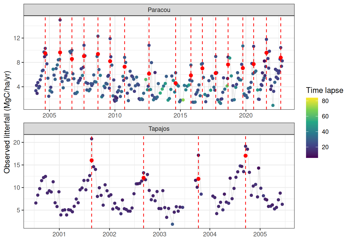
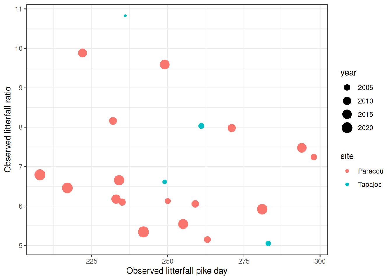
Paracou litterfall were provided by Damien Bonal (D. Bonal pers. com.). Tapajos litterfall are available online through the Oak Ridge National Laboratory (ORNL) Distributed Active Archive Center (DAAC): https://daac.ornl.gov/LBA/guides/CD10_Litter_Tapajos.html . Litterfall data were mainly used for the calibration of the new leaf phenology module in TROLL version 4. Leaf litterfall data were converted in fluxes over a defined time lag (depending on site and sampling date). For calibration two indices were derived for each years:
Day of the litterfall pike as the day of the maximum annual value
The litterfall rate is the ratio between the pike value (average of the annual maximum value and the previous and following values) divided by the base flow (average values between January and April)
read_tsv("outputs/litter.tsv") %>%ggplot(aes(date, litterfall, col = dt)) +geom_line(col ="lightgrey", alpha =0.5) +geom_point() +theme_bw() +facet_wrap(~ site, scales ="free", nrow =2) +scale_color_viridis_c("Time lapse") +xlab("") +ylab("Observed litterfall (MgC/ha/yr)") +geom_vline(aes(xintercept = pike_date), data = obs_metrics, col ="red", linetype ="dashed") +geom_point(aes(x = pike_date, y = pike), data = obs_metrics, col ="red", size =2)
Fortnightly measurement of litterfall at Tapajos and Paracou. Time lapse between two sampling is over 15-days for few measurement indicated by point colour. Annual pike of litterfall are indicated by the red lines and thier value by the red points.
Code
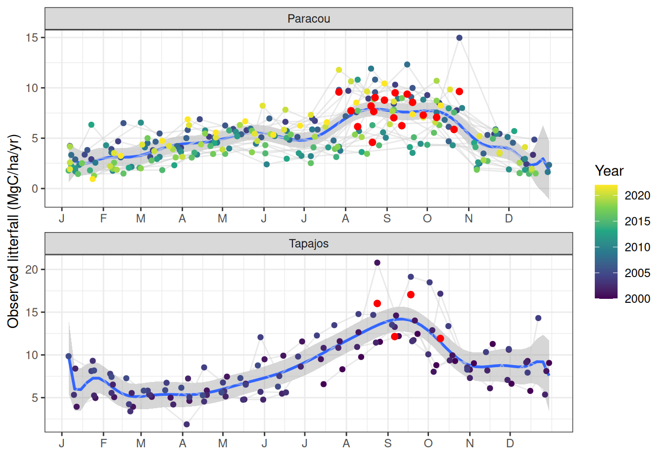
read_tsv("outputs/litter.tsv") %>%ggplot(aes(yday(date), litterfall, col =year(date))) +geom_smooth(method ="lm", formula = y ~poly(x, 20, raw =TRUE)) +geom_line(aes(group =as.factor(year(date))), col ="lightgrey", alpha =0.5) +geom_point() +theme_bw() +facet_wrap(~ site, scales ="free", nrow =2) +scale_color_viridis_c("Year") +xlab("") +ylab("Observed litterfall (MgC/ha/yr)") +scale_x_continuous(breaks =yday(as_date(paste0("2001-", 1:12, "-1"))),labels =c("J", "F", "M", "A", "M", "J", "J", "A", "S", "O", "N", "D")) +geom_point(aes(x = pike_day, y = pike), data = obs_metrics, col ="red", size =2)
Annual cycle of fortnightly measurement of litterfall at Tapajos and Paracou. Annual pike of litterfall are indicated by the red point.
Relations betweens Litterfall pike date and ratioi across years at Paracou and Tapajos.
Canopy structure
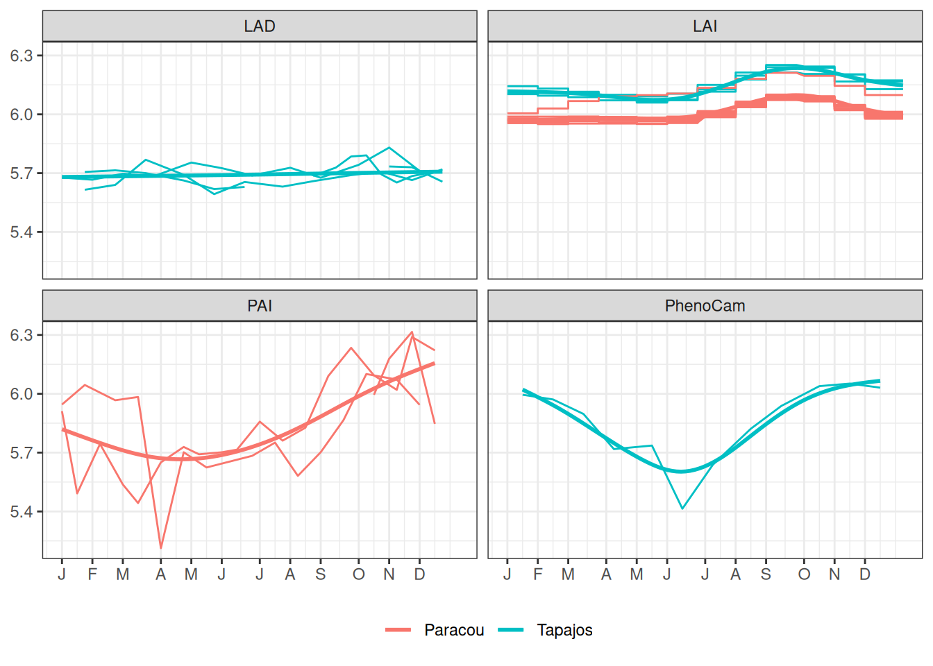
Canopy structure and dynamics was assessed using Leaf Area Index (LAI), Leaf Area Density (LAD) and Plant Area Density (PAD) from local observation using terrestrial or drone LIDAR remotely-sensed by MODIS. LIDAR data includes drone data from Paracou provided by Nicolas Barbier Bonal (G. Vincent & N. Barbier pers. com.) and terrestrial data from Tapajos etrieved from Smith et al. (2019): https://nph.onlinelibrary.wiley.com/doi/10.1111/nph.15726. Remotely-sensed data from MODIS were retrieved from PLUMBER2 on Research Data Australia: https://researchdata.edu.au/plumber2-forcing-evaluation-surface-models/1656048. Leaf area index was also extracted from PhenoCam of Wu et al. (2017) by X. Chen (pers. com.). Leaf area index per leaf cohort (LAI_age) was retrieved from Yang et al. (2023), from PhenoCam of Wu et al. (2017) by X. Chen (pers. com.), and reanalaysed by X. Chen et al. (in prep).
Annual cycle of leaf area density variation at Paracou and Tapajos measured every 8-days by satellite (LAI) across ten years, every 15-days by drone in Paracou across three years, or every 15-days at Tapajos from the ground in Tapajos for three years or from PhenoCam in Tapajos for one year (Wu et al. 2016).
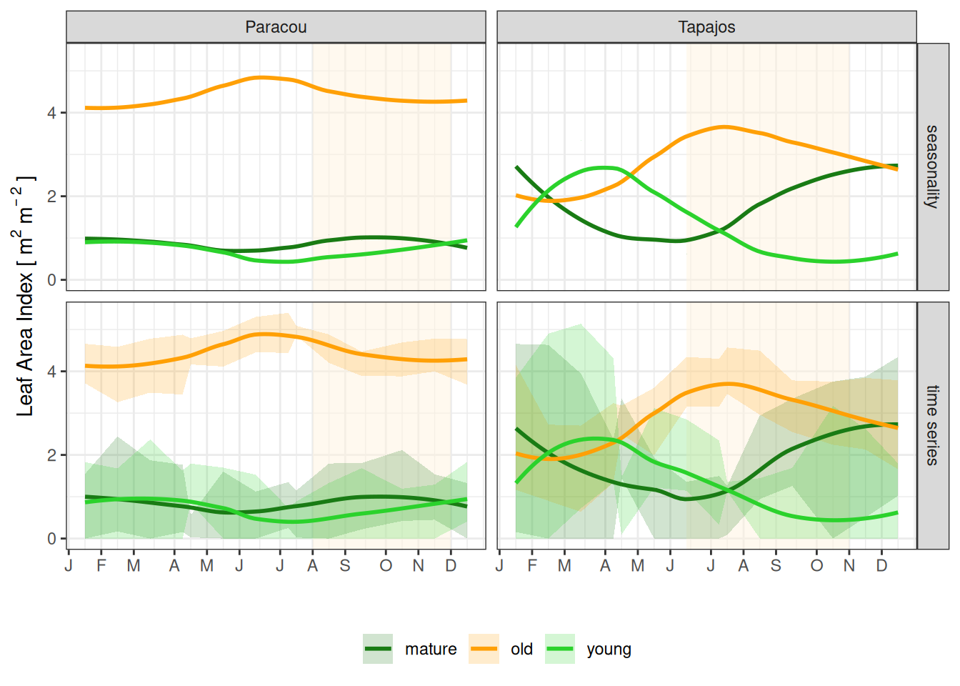
Mean annual cycle from fortnightly means of leaf area index for Paracou and Tapajos with leaf cohorts of yound, mature and old leaves from Yang et al. (2023). Bands are the intervals of means across years, and rectangles in the background correspond to the site’s climatological dry season.
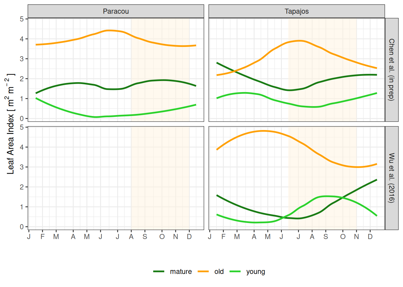
Mean annual cycle from monthlu means of leaf area index for Paracou and Tapajos with leaf cohorts of yound, mature and old leaves from PhenoCam of Wu et al. (2017) by X. Chen (pers. com.), and reanalaysed by X. Chen et al. (in prep). Rectangles in the background correspond to the site’s climatological dry season.
BONAL, DAMIEN, ALEXANDRE BOSC, STÉPHANE PONTON, JEAN-YVES GORET, BENOÎT BURBAN, PATRICK GROSS, JEAN-MARC BONNEFOND, et al. 2008. “Impact of Severe Dry Season on Net Ecosystem Exchange in the Neotropical Rainforest of French Guiana.”Global Change Biology 14 (8): 1917–33. https://doi.org/10.1111/j.1365-2486.2008.01610.x.
Chen, Xingan, Yuefei Huang, Chong Nie, Shuo Zhang, Guangqian Wang, Shiliu Chen, and Zhichao Chen. 2022. “A Long-Term Reconstructed TROPOMI Solar-Induced Fluorescence Dataset Using Machine Learning Algorithms.”Scientific Data 9 (1). https://doi.org/10.1038/s41597-022-01520-1.
Pastorello, Gilberto, Trotta, Carlo, Canfora, Eleonora, Chu, Housen, Christianson, Danielle, Cheah, You-Wei, Poindexter, Cristina, et al. 2020. “The FLUXNET2015 Dataset and the ONEFlux Processing Pipeline for Eddy Covariance Data.”Nature Publishing Group. https://doi.org/10.5167/UZH-190509.
Smith, Marielle N., Scott C. Stark, Tyeen C. Taylor, Mauricio L. Ferreira, Eronaldo de Oliveira, Natalia Restrepo-Coupe, Shuli Chen, et al. 2019. “Seasonal and Drought-Related Changes in Leaf Area Profiles Depend on Height and Light Environment in an Amazon Forest.”New Phytologist 222 (3): 1284–97. https://doi.org/10.1111/nph.15726.
Ukkola, Anna M., Gab Abramowitz, and Martin G. De Kauwe. 2022. “A Flux Tower Dataset Tailored for Land Model Evaluation.”Earth System Science Data 14 (2): 449–61. https://doi.org/10.5194/essd-14-449-2022.
Wu, Jin, Loren P. Albert, Aline P. Lopes, Natalia Restrepo-Coupe, Matthew Hayek, Kenia T. Wiedemann, Kaiyu Guan, et al. 2017. “Data from: Leaf Development and Demography Explain Photosynthetic Seasonality in Amazon Evergreen Forests.” Dryad. https://doi.org/10.5061/DRYAD.8FB47.
Yang, Xueqin, Xiuzhi Chen, Jiashun Ren, Wenping Yuan, Liyang Liu, Juxiu Liu, Dexiang Chen, et al. 2023. “A Grid Dataset of Leaf Age-Dependent LAI Seasonality Product (Lad-LAI) over Tropical and Subtropical Evergreen Broadleaved Forests.”http://dx.doi.org/10.5194/essd-2022-436.