Variation

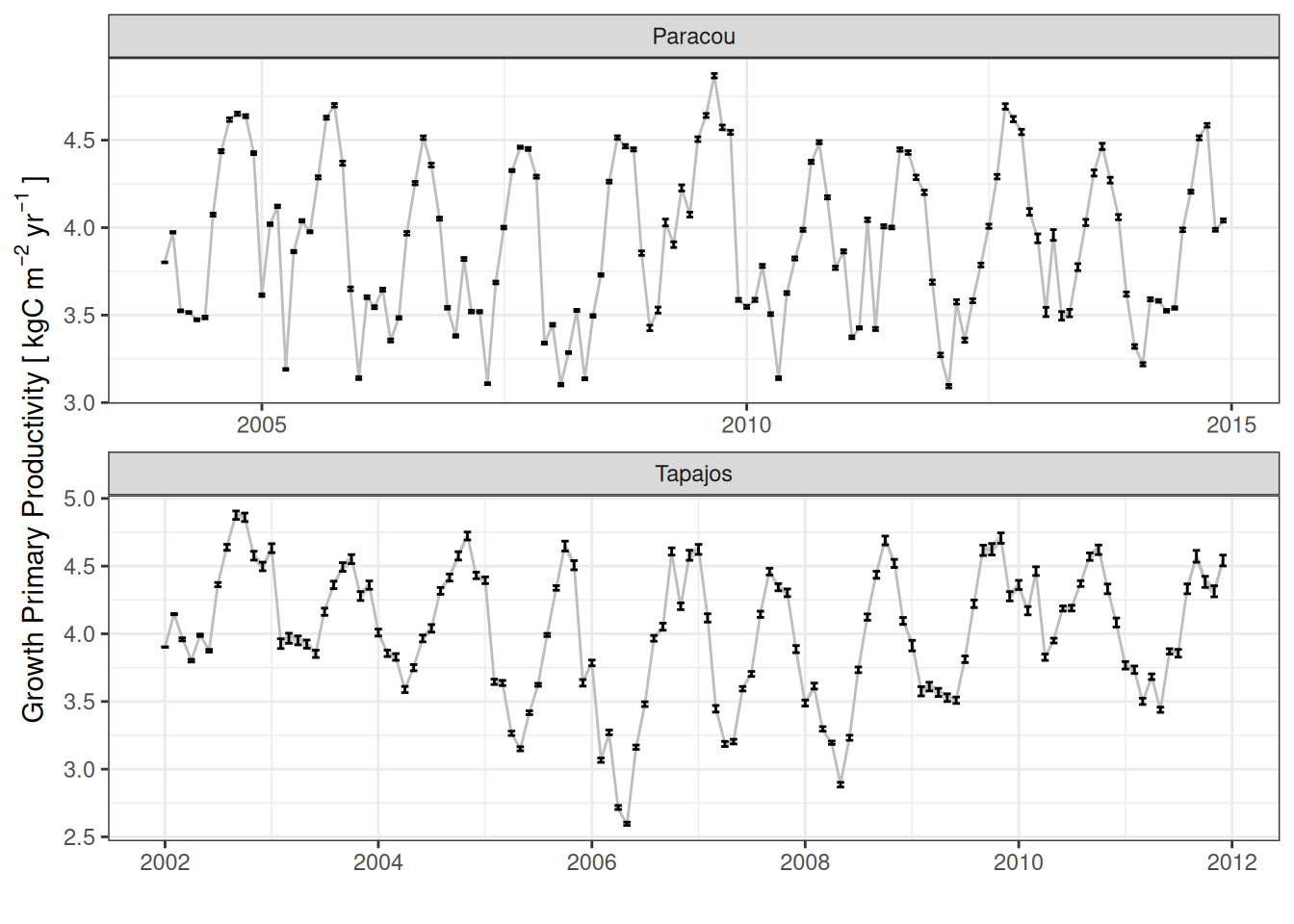
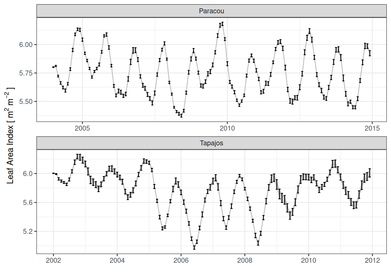
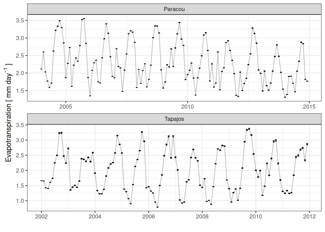
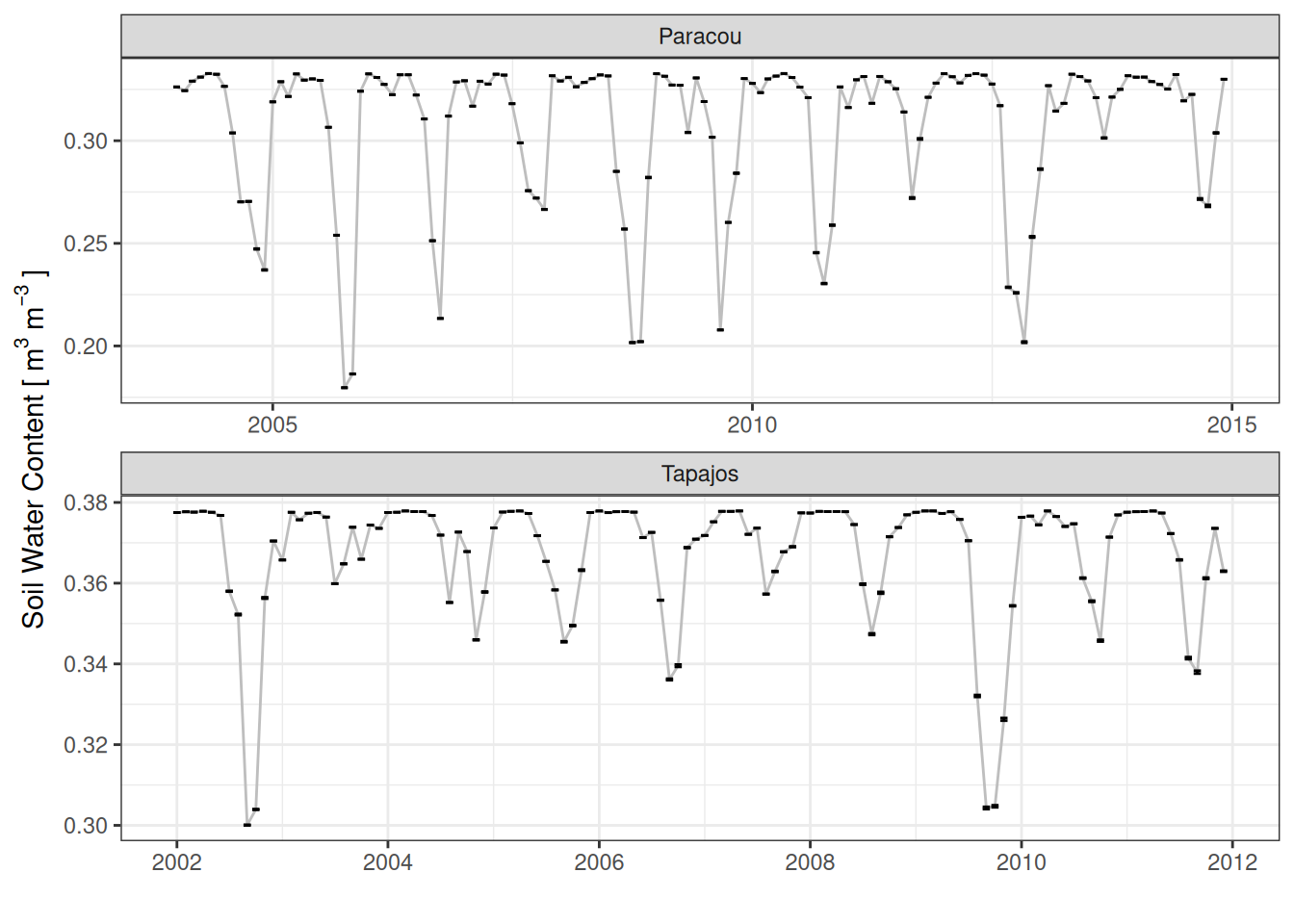
TROLL simulations showed very little variations due to stochasticity in fluxes (however this is 10-years variations starting from a single spin-up). The highest variation is in Leaf Area Index (LAI, m2/m2), partly due to higher possible stochasticity in leaf shedding, but remains negligible. Oppositely, Growth Primary Productivity (GPP, kgC/m2/yr), evapotranspiration (ET, mm/day) and Soil Water Content (SWC, m3/m3) showed almost no-variations across simulations of monthly mean values.

Code

files <- list.files("results/eval/", pattern = "sumstats.txt", 
                    recursive = T, full.names = T) 
names(files) <- list.files("results/eval/", pattern = "sumstats.txt", 
                    recursive = T, full.names = F) 
period <- "month"
files %>% 
  lapply(vroom::vroom) %>% 
  bind_rows(.id = "file") %>% 
  separate(file, "sim", "/") %>% 
  separate(sim, c("site", "repetition")) %>%
  mutate(repetition = as.numeric(gsub("R", "", repetition))) %>% 
  mutate(gpp = gpp*10^2*365/10^3) %>% 
  select(site, repetition, iter, gpp) %>% 
  mutate(date = as_date(ifelse(site == "Paracou", 
                       "2004/01/01", 
                       "2002/01/01"))) %>% 
  mutate(date = date + iter) %>% 
  group_by(site, repetition, date = floor_date(date, period)) %>% 
  summarise(gpp = mean(gpp)) %>% 
  group_by(site, date = floor_date(date, period)) %>% 
  summarise(l = min(gpp), 
            m = median(gpp), 
            h = max(gpp)) %>% 
  ggplot(aes(date, m)) +
  geom_ribbon(aes(ymin = l, ymax = h), col = NA, alpha = 0.2) +
  geom_line(col = "grey") +
  geom_errorbar(aes(ymin = l, ymax = h)) +
  facet_wrap(~ site, nrow = 2, scales = "free") +
  theme_bw() +
  xlab("") +
  ylab(expression("Growth Primary Productivity ["~kgC~m^{-2}~yr^{-1}~"]")) 

Variability of monthly means of growth primary productivity for Paracou and Tapajos across 10 TROLL simulations.

Code

files <- list.files("results/eval/", pattern = "LAIdynamics.txt", 
                    recursive = T, full.names = T) 
names(files) <- list.files("results/eval/", pattern = "LAIdynamics.txt", 
                    recursive = T, full.names = F) 
period <- "month"
files %>% 
  lapply(vroom::vroom) %>% 
  bind_rows(.id = "file") %>% 
  separate(file, "sim", "/") %>% 
  separate(sim, c("site", "repetition")) %>%
  mutate(repetition = as.numeric(gsub("R", "", repetition))) %>% 
  mutate(date = as_date(ifelse(site == "Paracou", 
                       "2004/01/01", 
                       "2002/01/01"))) %>% 
  mutate(date = date + iter) %>% 
  group_by(site, repetition, date = floor_date(date, period)) %>% 
  summarise(LAI = mean(LAI)) %>% 
  group_by(site, date = floor_date(date, period)) %>% 
  summarise(l = min(LAI), 
            m = median(LAI), 
            h = max(LAI)) %>% 
  ggplot(aes(date, m)) +
  geom_ribbon(aes(ymin = l, ymax = h), col = NA, alpha = 0.2) +
  geom_line(col = "grey") +
  geom_errorbar(aes(ymin = l, ymax = h)) +
  facet_wrap(~ site, nrow = 2, scales = "free") +
  theme_bw() +
  xlab("") + 
  ylab(expression("Leaf Area Index ["~m^2~m^{-2}~"]")) 

Variability of monthly means of leaf area index for Paracou and Tapajos across 10 TROLL simulations.

Code

files <- list.files("results/eval/", pattern = "water_balance.txt", 
                    recursive = T, full.names = T) 
names(files) <- list.files("results/eval/", pattern = "water_balance.txt", 
                    recursive = T, full.names = F) 
period <- "month"
files %>% 
  lapply(vroom::vroom) %>% 
  bind_rows(.id = "file") %>% 
  separate(file, "sim", "/") %>% 
  separate(sim, c("site", "repetition")) %>%
  mutate(repetition = as.numeric(gsub("R", "", repetition))) %>% 
  mutate(date = as_date(ifelse(site == "Paracou", 
                       "2004/01/01", 
                       "2002/01/01"))) %>% 
  mutate(date = date + iter) %>% 
  mutate(et = (transpitation_0 + transpitation_1 + transpitation_2 + 
                 transpitation_3 + transpitation_4 + evaporation)*1000) %>% 
  group_by(site, repetition, date = floor_date(date, period)) %>% 
  summarise(et = mean(et)) %>% 
  group_by(site, date = floor_date(date, period)) %>% 
  summarise(l = min(et), 
            m = median(et), 
            h = max(et)) %>% 
  ggplot(aes(date, m)) +
  geom_ribbon(aes(ymin = l, ymax = h), col = NA, alpha = 0.2) +
  geom_line(col = "grey") +
  geom_errorbar(aes(ymin = l, ymax = h)) +
  facet_wrap(~ site, nrow = 2, scales = "free") +
  theme_bw() +
  xlab("") + 
  ylab(expression("Evapotranspiration ["~mm~day^{-1}~"]")) 

Variability of monthly means of evapotranspiration for Paracou and Tapajos across 10 TROLL simulations.

Code

files <- list.files("results/eval/", pattern = "water_balance.txt", 
                    recursive = T, full.names = T) 
names(files) <- list.files("results/eval/", pattern = "water_balance.txt", 
                    recursive = T, full.names = F) 
period <- "month"
files %>% 
  lapply(vroom::vroom) %>% 
  bind_rows(.id = "file") %>% 
  separate(file, "sim", "/") %>% 
  separate(sim, c("site", "repetition")) %>%
  mutate(repetition = as.numeric(gsub("R", "", repetition))) %>% 
  mutate(date = as_date(ifelse(site == "Paracou", 
                       "2004/01/01", 
                       "2002/01/01"))) %>% 
  mutate(date = date + iter) %>% 
  group_by(site, repetition, date = floor_date(date, period)) %>% 
  summarise(SWC_0 = mean(SWC_0)) %>% 
  group_by(site, date = floor_date(date, period)) %>% 
  summarise(l = min(SWC_0), 
            m = median(SWC_0), 
            h = max(SWC_0)) %>% 
  ggplot(aes(date, m)) +
  geom_ribbon(aes(ymin = l, ymax = h), col = NA, alpha = 0.2) +
  geom_line(col = "grey") +
  geom_errorbar(aes(ymin = l, ymax = h)) +
  facet_wrap(~ site, nrow = 2, scales = "free") +
  theme_bw() +
  xlab("") + 
  ylab(expression("Soil Water Content ["~m^{3}~m^{-3}~"]")) 

Variability of monthly means of soil water content for Paracou and Tapajos across 10 TROLL simulations.