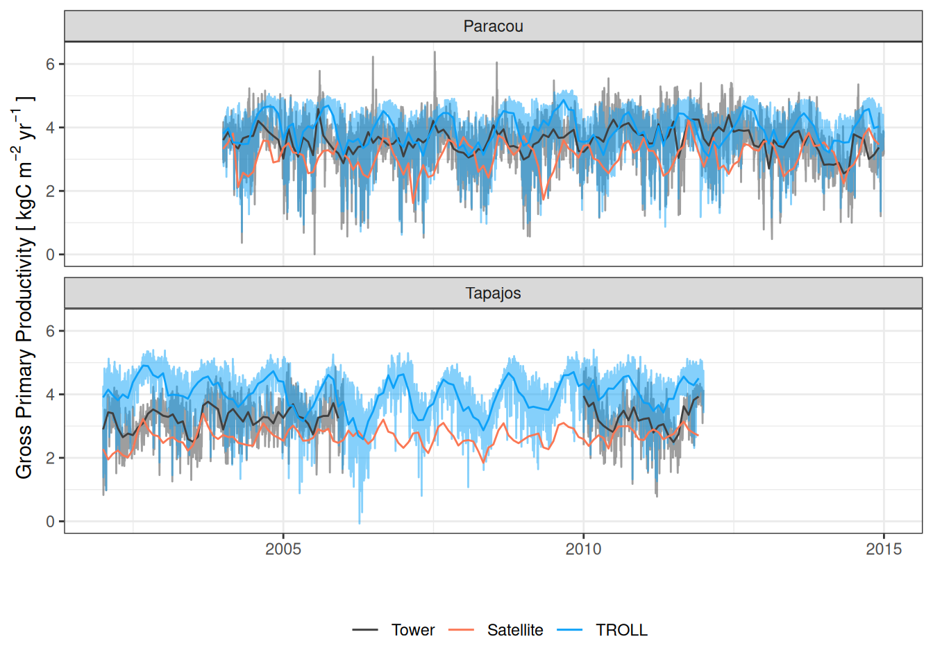
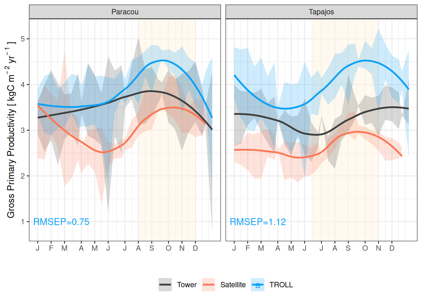
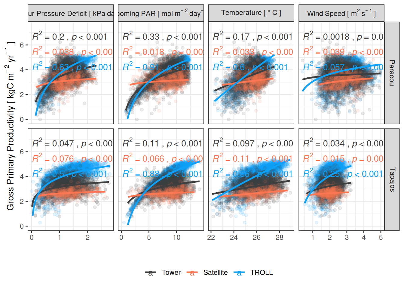
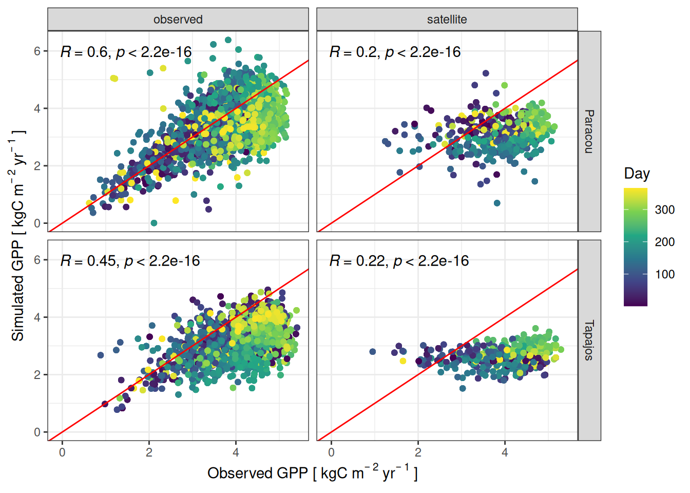
The new version of TROLL correctly simulated the phenology of Gross Primary Productivity (GPP, kgC/m2/yr) with a lower GPP in wet season and higher values in the dry season. However, TROLL version 4 is globally overestimating GPP with daily values overlapping wet season values but significantly higher values in dry season with a pike around 5 instead of 4 kgC/m2/yr. Remotely-sensed observation from TROPOMI Solar Induced Fluorescence showed under-estimated values of GPP between 2.5 and 3.5 kgC/m2/yr monthly means but with a similar phenology. The new version of TROLL seems to be too deterministic in the relation between available light (incoming PAR mol/m2/day) and GPP with a correlation coefficient of 0.94 against an observed coefficient of 0.58. The overestimation of GPP seems to be linked to over-efficient GPP for high light availability (PAR above 5 mol/m2/day). Globally, simulated GPP showed a very good evaluation with a correlation coefficient of 0.59 in Paracou and 0.46 in Tapajos against daily observations from eddy-flux towers, and corresponding RMSEP of respectively 0.9 and 1.6 kgC/m2/yr.
Daily and monthly means of growth primary productivity for Paracou and Tapajos. Dark lines are the monthly means, semi-transparent lines are the daily means variations with the exception of satellite data for which data are available only every 8 days.
Mean annual cycle from fortnightly means of growth primary productivity for Paracou and Tapajos. Bands are the intervals of means across years, and rectangles in the background correspond to the site’s climatological dry season.
Daily averages of growth primary productivity as a function of vapour pressure deficit, incoming photosynthetically active radiation, temperature, and wind speed for model-, satellite- and tower-based estimates at Paracou and Tapajos.
Evaluation of simulated versus observed daily means of GPP in Paracou and Tapajos.
Code
daily %>%pivot_wider(names_from = type, values_from = value) %>%gather(type, observed, -site, -date, -variable, -determinant, -determinant_value, -simulated) %>%na.omit() %>%nest_by(site, variable, type) %>%mutate(R2 =summary(lm(observed ~0+ simulated, data = data))$r.squared,CC =cor(data$simulated, data$observed),RMSEP =sqrt(mean((data$simulated-data$observed)^2)),RRMSEP =sqrt(mean((data$simulated-data$observed)^2))/mean(data$observed),SD =sd(data$simulated-data$observed),RSD =sd(data$simulated-data$observed)/mean(data$observed)) %>%select(-data) %>% knitr::kable(caption ="Evaluation fo daily means of GPP at Paracou and Tapajos.")
Evaluation fo daily means of GPP at Paracou and Tapajos.
site
variable
type
R2
CC
RMSEP
RRMSEP
SD
RSD
Paracou
gpp
observed
0.9697223
0.6038441
0.743844
0.2078451
0.6658932
0.1860641
Paracou
gpp
satellite
0.9535270
0.1980375
1.169922
0.3775626
0.7935245
0.2560900
Tapajos
gpp
observed
0.9674821
0.4546221
1.124531
0.3486050
0.6763800
0.2096780
Tapajos
gpp
satellite
0.9615592
0.2199041
1.541116
0.5816081
0.7538847
0.2845117
Leaf Area Index
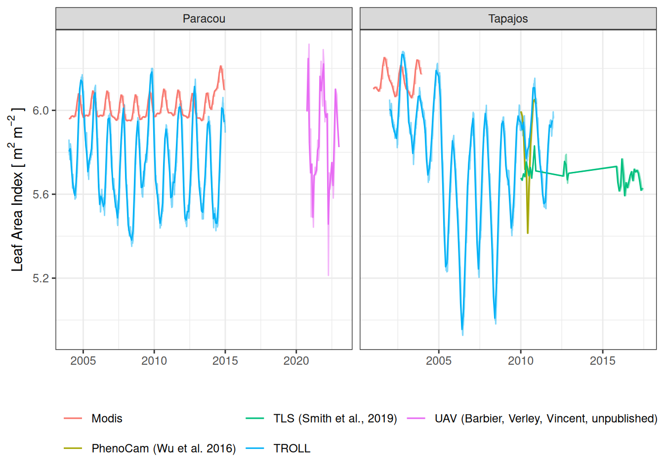
We had multiples data to evaluate canopy dynamics and resulting Leaf Area Index (LAI, m2/m2) that were not in agreement and unfortunately not in the same time period. LAI from MODIS shows a base value around 6 m2/m2 most of the years and a small increase below 0.2 m2/m3 in the dry season that pike in the middle of the dry season at both Paracou and Tapajos. Field measures with drone lidar showed a greater variation in Paracou with lowest values of 5.5 m2/m2 in April to June and highest values of almost 6 m2/m2 in December. Oppositely, field measures with terrestrial lidar in Tapajos showed no variation of LAI stable around 5.75 m2/m2 the whole year. This results thus question the use of MODIS LAI for TROLL evaluation. Indeed simulated LAI followed also the same phenology with an crease of LAI during the dry season but with values matching drone data in Paracou and not MODIS product. In Tapajos, the simulations showed even higher variations of LAI, that did not correspond to both MODIS and terrestrial LAD. Globally, simulated LAI showed a weak evaluation with a correlation coefficient of 0.37 in Paracou and 0.63 in Tapajos against 8-day observations from MODIS satellites, and corresponding RMSEP of respectively 0.3 and 0.1 m2/m2.
Code
daily <-read_tsv("outputs/evaluation_fluxes.tsv") %>%filter(variable =="lai") %>%select(-variable) %>%mutate(type ="simulated") %>%rename(value = simulated) %>%bind_rows(read_tsv("outputs/lai.tsv") %>%rename(type = variable)) %>%bind_rows(readxl::read_xlsx("data/fluxes/Data_LAI_new.xlsx") %>%mutate(date =as_date(paste0("2010-", month, "-15"))) %>%mutate(site ="Tapajos", type ="PhenoCam", value =`Camera_LAI (m^2 m^-2)`) %>%select(date, value, site, type)) %>%mutate(type =recode(type, "LAD"="TLS (Smith et al., 2019)","LAI"="Modis","PAI"="UAV (Barbier, Verley, Vincent, unpublished)","PhenoCam"="PhenoCam (Wu et al. 2016)","simulated"="TROLL"))monthly <- daily %>%group_by(site, date =floor_date(date, "month"), type) %>%summarise(l =quantile(value, 0.025, na.rm =TRUE), value =mean(value, na.rm =TRUE), h =quantile(value, 0.975, na.rm =TRUE))
Code
daily %>%ggplot(aes(date, value, col = type)) +geom_line(alpha =0.5) +geom_line(data = monthly) +facet_wrap(~ site, scales ="free_x") +theme_bw() +theme(legend.position ="bottom") +xlab("") +ylab(expression("Leaf Area Index ["~m^2~m^{-2}~"]")) +scale_color_discrete("") +guides(col =guide_legend(nrow =2))
Daily and monthly means of leaf area index for Paracou and Tapajos. Dark lines are the monthly means, semi-transparent lines are the daily means variations with the exception of satellite data for which data are available only every 8 days.
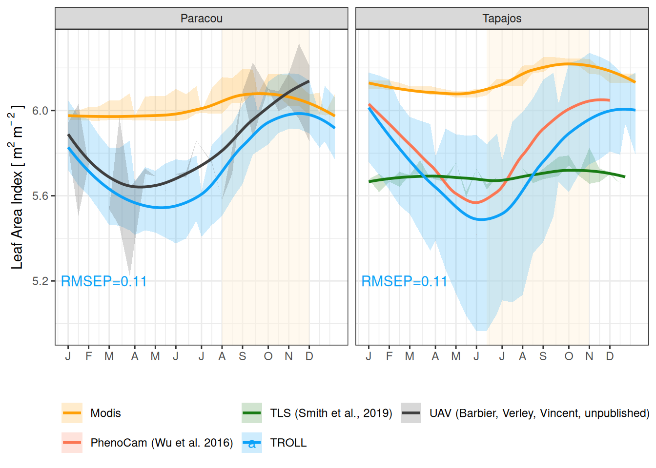
Mean annual cycle from fortnightly means of leaf area index for Paracou and Tapajos. Bands are the intervals of means across years, and rectangles in the background correspond to the site’s climatological dry season.
Code
daily %>%group_by(site, type, date =floor_date(date, "15 days")) %>%summarise_all(mean, na.rm = T) %>%mutate(week =week(date)) %>%group_by(site, type, week) %>%summarise(value =mean(value, na.rm =TRUE)) %>%pivot_wider(names_from = type, values_from = value) %>%rename(simulated = TROLL) %>%gather(type, observed, -site, -week, -simulated) %>%na.omit() %>%ungroup() %>%nest_by(site, type) %>%mutate(R2 =summary(lm(observed ~0+ simulated, data = data))$r.squared,CC =cor(data$simulated, data$observed),RMSEP =sqrt(mean((data$simulated-data$observed)^2)),RRMSEP =sqrt(mean((data$simulated-data$observed)^2))/mean(data$observed),SD =sd(data$simulated-data$observed),RSD =sd(data$simulated-data$observed)/mean(data$observed)) %>%select(-data) %>% knitr::kable(caption ="Evaluation fo monthly means of LAI at Paracou and Tapajos.")
Evaluation fo monthly means of LAI at Paracou and Tapajos.
site
type
R2
CC
RMSEP
RRMSEP
SD
RSD
Paracou
Modis
0.9993110
0.6443293
0.2995714
0.0498207
0.1528940
0.0254273
Paracou
UAV (Barbier, Verley, Vincent, unpublished)
0.9996465
0.8404994
0.1378908
0.0236607
0.1121080
0.0192366
Tapajos
Modis
0.9992162
0.5613419
0.3990495
0.0649692
0.1641144
0.0267195
Tapajos
PhenoCam (Wu et al. 2016)
0.9998312
0.9169373
0.1124293
0.0192047
0.0790174
0.0134974
Tapajos
TLS (Smith et al., 2019)
0.9990079
0.2484052
0.2014810
0.0353875
0.1859247
0.0326553
Leaf Area Index per Age
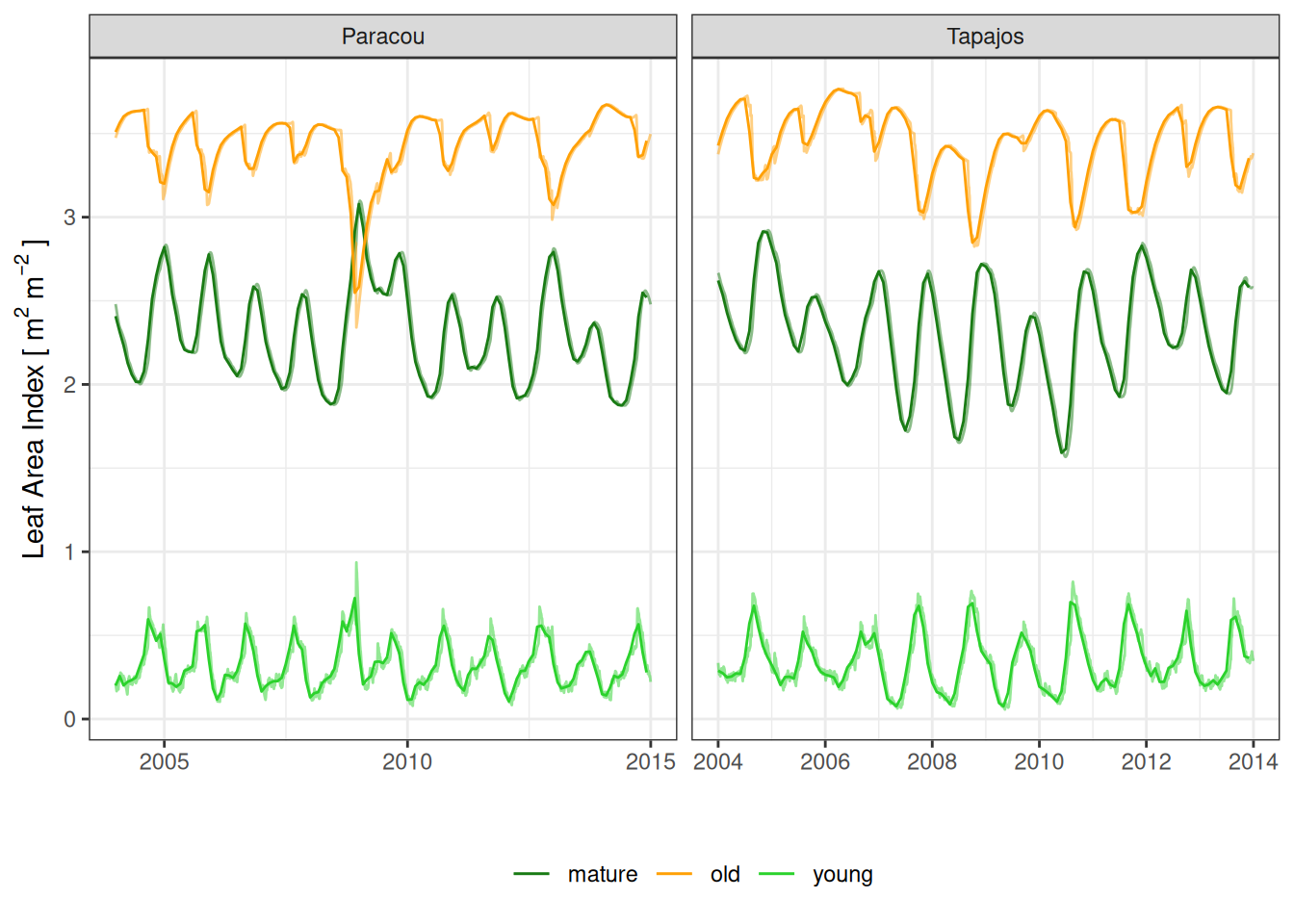
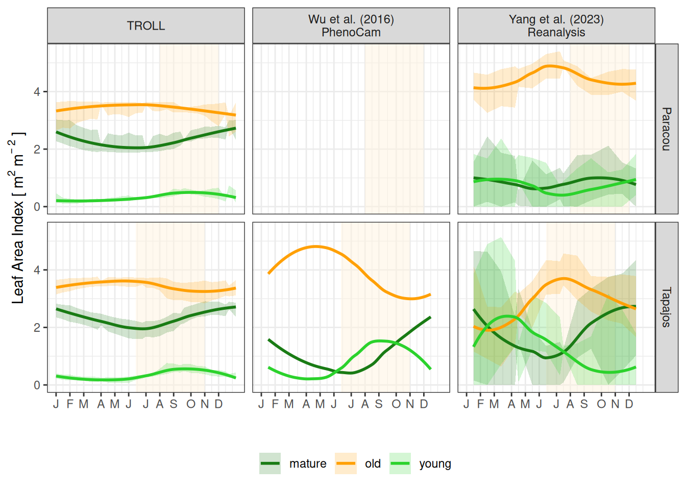
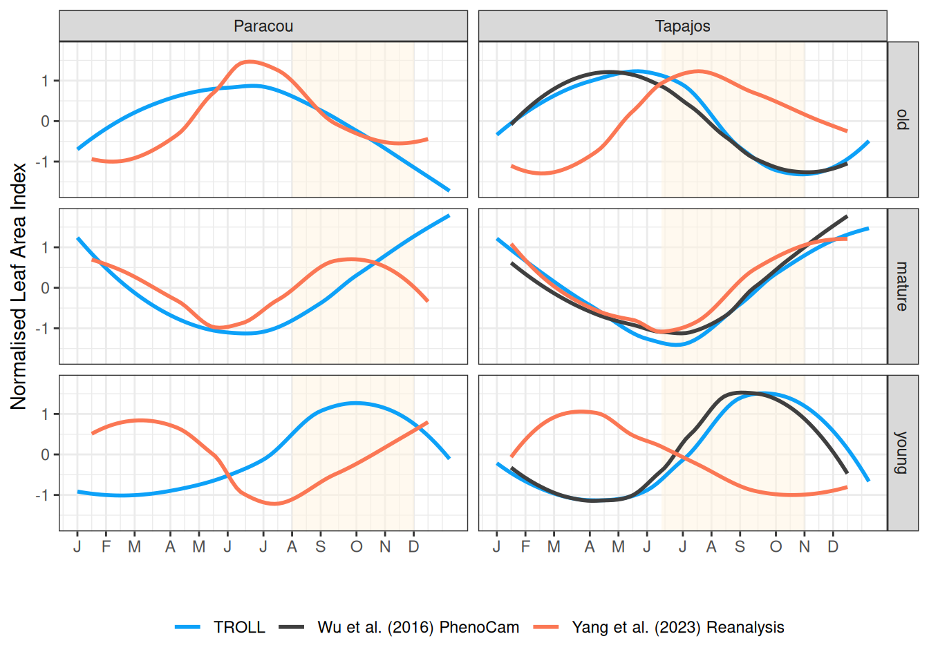
For comparisons with Yang et al. (2023), we also simulated Leaf Area Index per leaf-age class. In the figure 8 of Yang et al. (2023) Tapajos is represented by the subclass S1, characterised by an always higher values old LAI above 3 m2/m2 and lower values of young and mature LAI around 1.5 m2/m2, while Paracou is represented by the subclass S2, characterised with high values of old LAI and low value of young and mature LAI in wet season but a strong loss of old LAI, a strong increase in mature LAI, a slight increase of young LAI in dry season. Similarly, in our simulations we observed a high LAI of old leaves especially in Tapajos. It seems that old leaf area are overestimated in Tapajos, because a priori there is little interest in accumulating less efficient leaves, and therefore confirms the hypothesis that the basal flux of litter is not high enough for Tapajos. At Paracou, we simulated back the phenology of Yang et al. (2023) with increased young LAI and mature LAI in the dry season while old LAI is decreasing, but a bit later than in Yang et al. (2023) and with values of mature LAI similar to those of old LAI between 2 and 3.5 m2/m2.
daily %>%ggplot(aes(date, value, col = age)) +geom_line(alpha =0.5) +geom_line(data = monthly) +facet_wrap(~ site, scales ="free_x") +theme_bw() +theme(legend.position ="bottom") +xlab("") +ylab(expression("Leaf Area Index ["~m^2~m^{-2}~"]")) +scale_color_manual("", values =as.vector(cols_laid[c("mature", "old", "young")]))
Daily and monthly means of leaf area index for Paracou and Tapajos with leaf cohorts of yound, mature and old leaves. Dark lines are the monthly means, semi-transparent lines are the daily means variations.
Mean annual cycle from fortnightly means of leaf area index for Paracou and Tapajos with leaf cohorts of yound, mature and old leaves. Bands are the intervals of means across years, and rectangles in the background correspond to the site’s climatological dry season.
Mean annual cycle from fortnightly means of leaf area index for Paracou and Tapajos with leaf cohorts of yound, mature and old leaves. Bands are the intervals of means across years, and rectangles in the background correspond to the site’s climatological dry season.
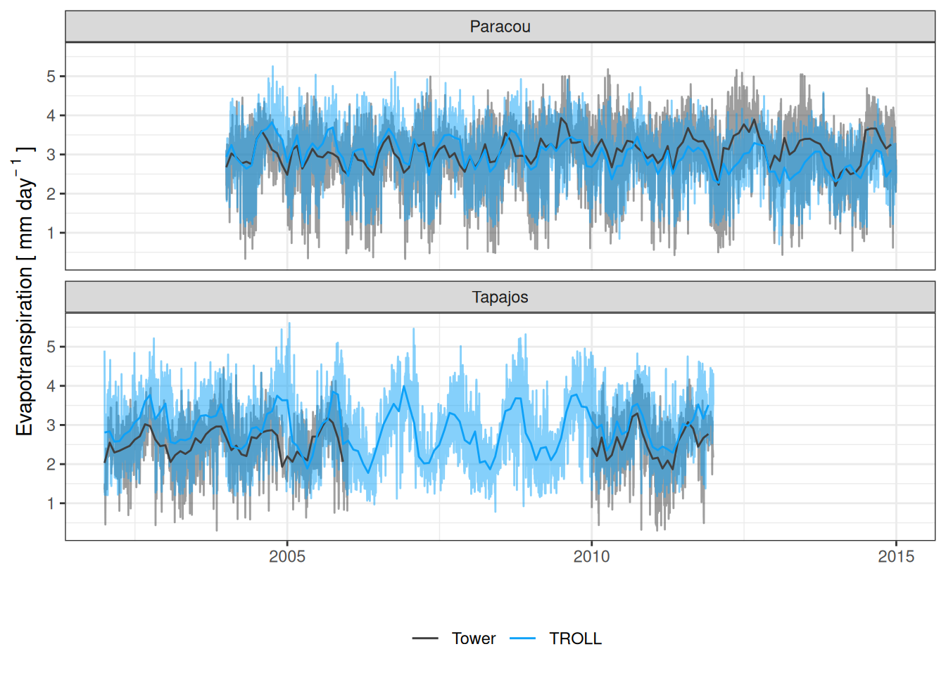
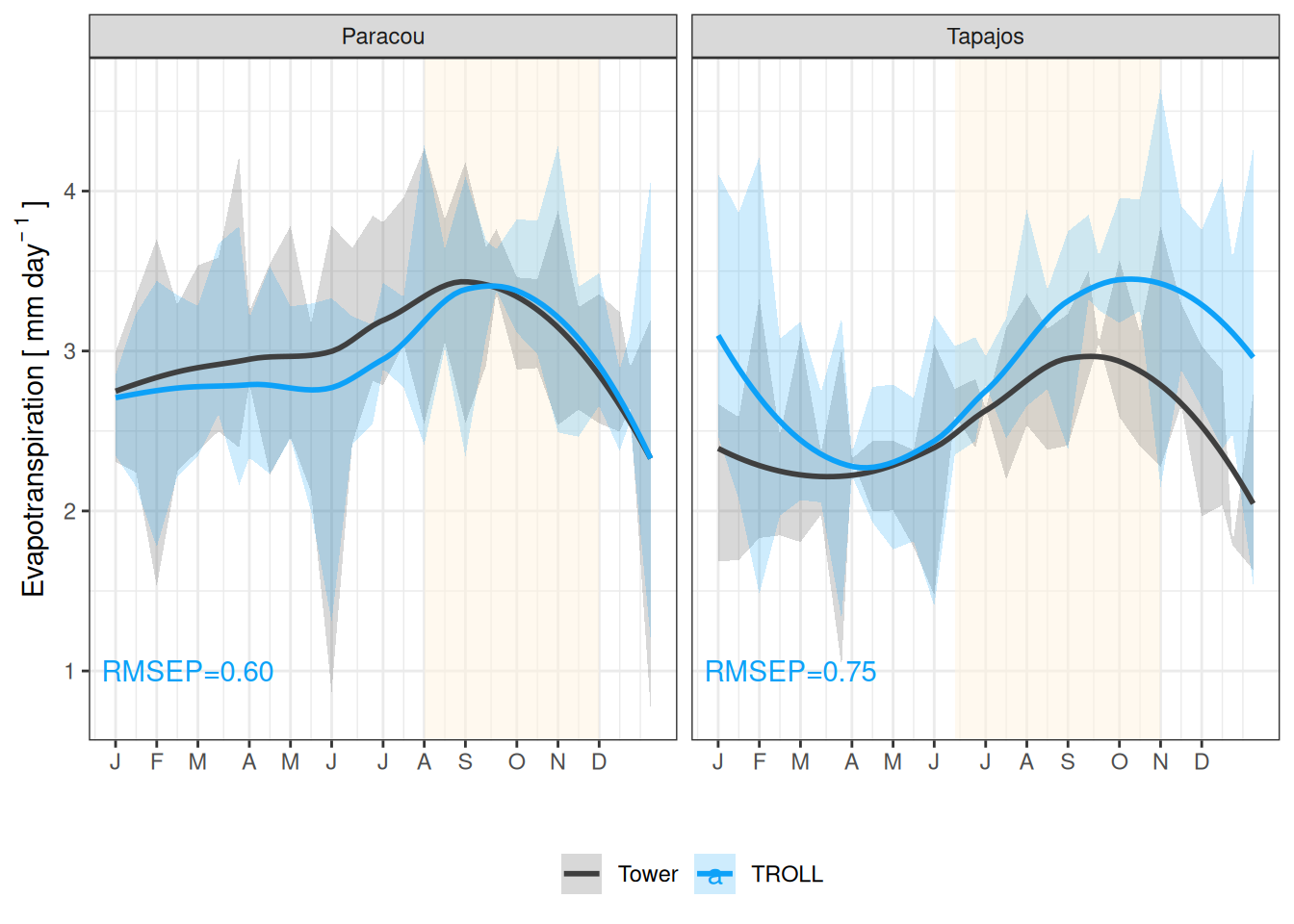
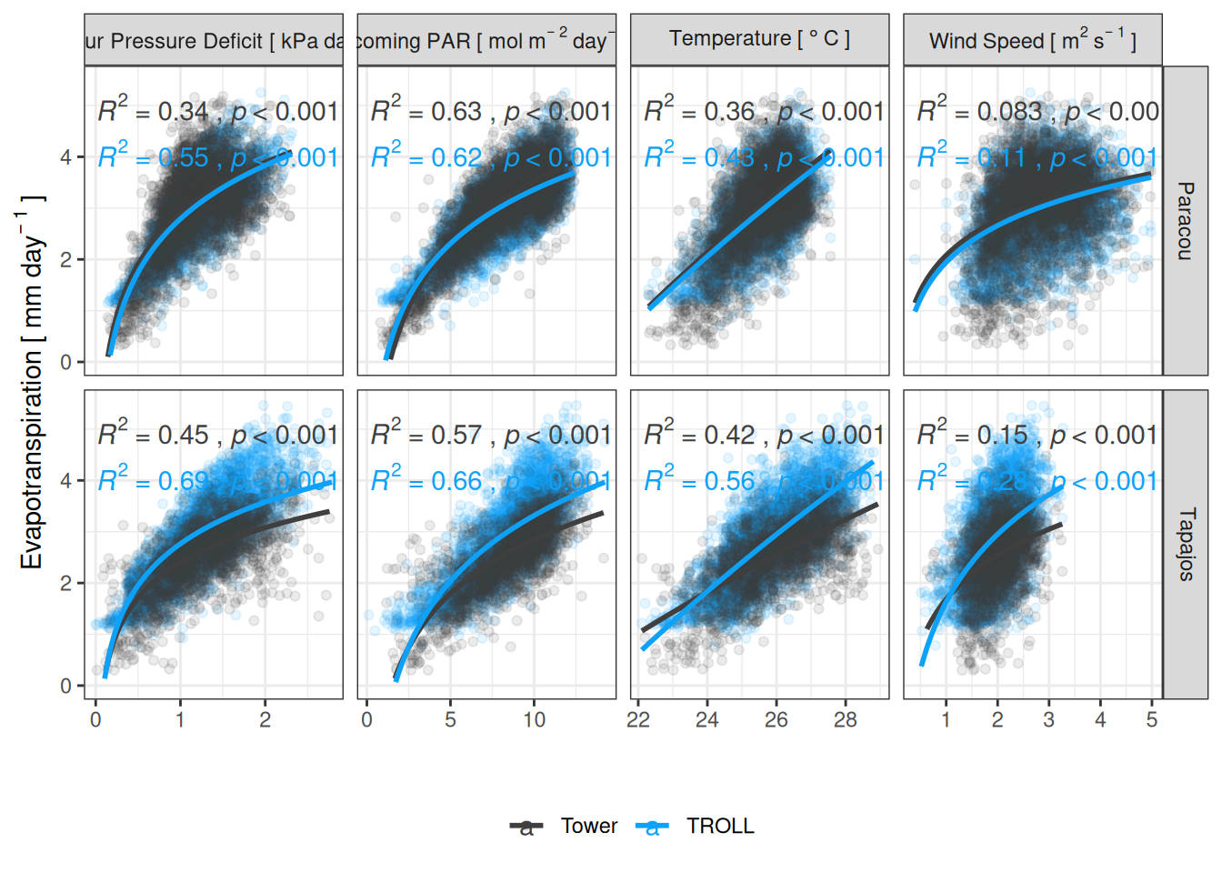
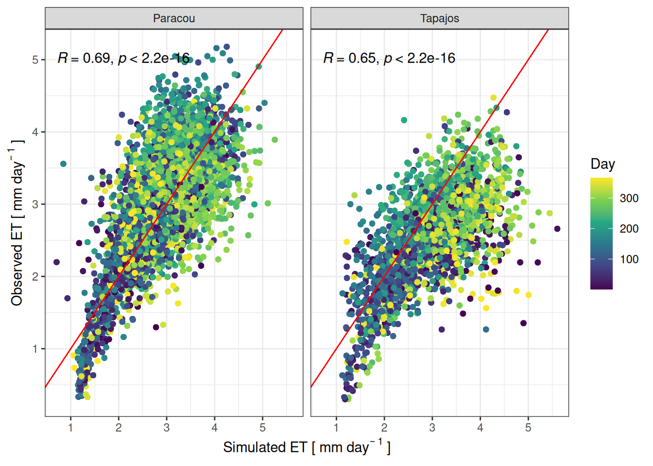
The new version of TROLL correctly simulated the phenology of evapotranspiration (ET, mm/day), with a lower ET in wet season and an higher evaporative demand in the dry season. Simulations are slightly underestimating the ET but globally daily values overlaps in most of the 15-days windows with a wet season flux simulated around 2 mm/day against 3 mm/day observed in Paracou and both around 3.5 mm/day in the dry season. Similarly in Tapajos, the wet season flux simulated drop to almost 1 mm/day despite being above 2 mm/day in observations and they both reach 3 mm/day in the dry season. Both simulations and observations are driven by daily maximum vapour pressure deficit with a correlation coefficient between 0.58 and 0.67 for observation, and more deterministic for simulations between 0.89 and 0.93. Globally, simulated ET showed a very good evaluation with a correlation coefficient of 0.73 in Paracou and 0.72 in Tapajos against daily observations from eddy-flux towers, and corresponding RMSEP of respectively 0.9 and 0.8 mm/day.
Daily and monthly means of evapotranpsiration for Paracou and Tapajos. Dark lines are the monthly means, semi-transparent lines are the daily means variations
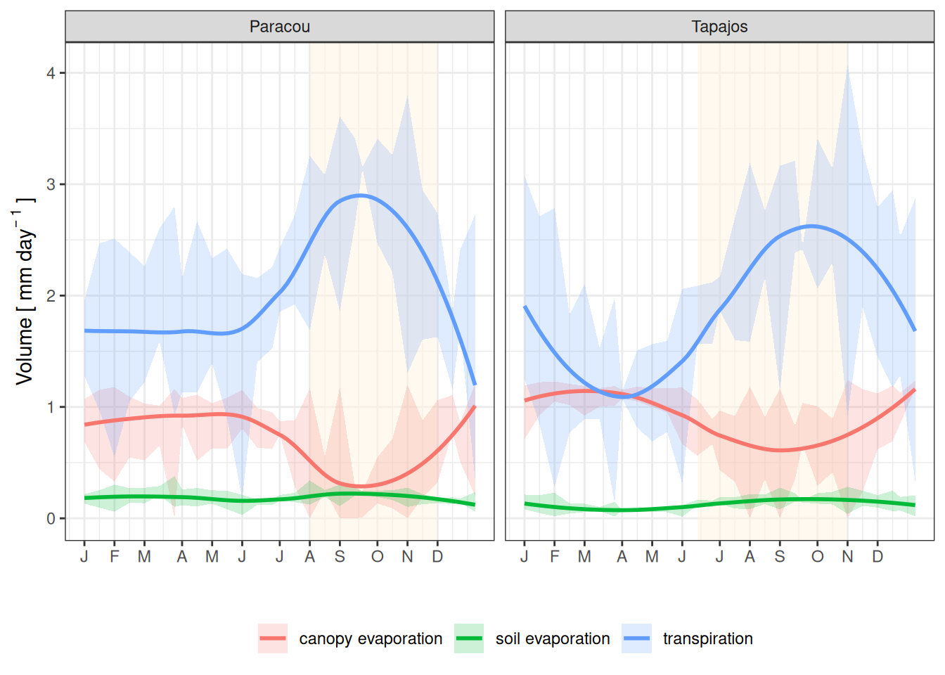
Mean annual cycle from fortnightly means of evapotranspiration for Paracou and Tapajos. Bands are the intervals of means across years, and rectangles in the background correspond to the site’s climatological dry season.
Daily averages of evapotranspiration as a function of vapour pressure deficit, incoming photosynthetically active radiation, temperature, and wind speed for model-, satellite- and tower-based estimates at Paracou and Tapajos.
Code
daily %>%pivot_wider(names_from = type, values_from = value) %>%ggplot(aes(simulated ,observed, col =yday(date))) +facet_wrap(~ site) +theme_bw() +geom_point() +scale_color_viridis_c("Day") +geom_abline(col ="red") +ylab(expression("Observed ET ["~mm~day^{-~1}~"]")) +xlab(expression("Simulated ET ["~mm~day^{-~1}~"]")) +scale_color_viridis_c("Day") + ggpubr::stat_cor()
Evaluation of simulated versus observed daily means of ET in Paracou and Tapajos.
Code
daily %>%pivot_wider(names_from = type, values_from = value) %>%na.omit() %>%nest_by(site, variable) %>%mutate(R2 =summary(lm(observed ~0+ simulated, data = data))$r.squared,CC =cor(data$simulated, data$observed),RMSEP =sqrt(mean((data$simulated-data$observed)^2)),RRMSEP =sqrt(mean((data$simulated-data$observed)^2))/mean(data$observed),SD =sd(data$simulated-data$observed),RSD =sd(data$simulated-data$observed)/mean(data$observed)) %>%select(-data) %>% knitr::kable(caption ="Evaluation fo daily means of ET at Paracou and Tapajos.")
Evaluation fo daily means of ET at Paracou and Tapajos.
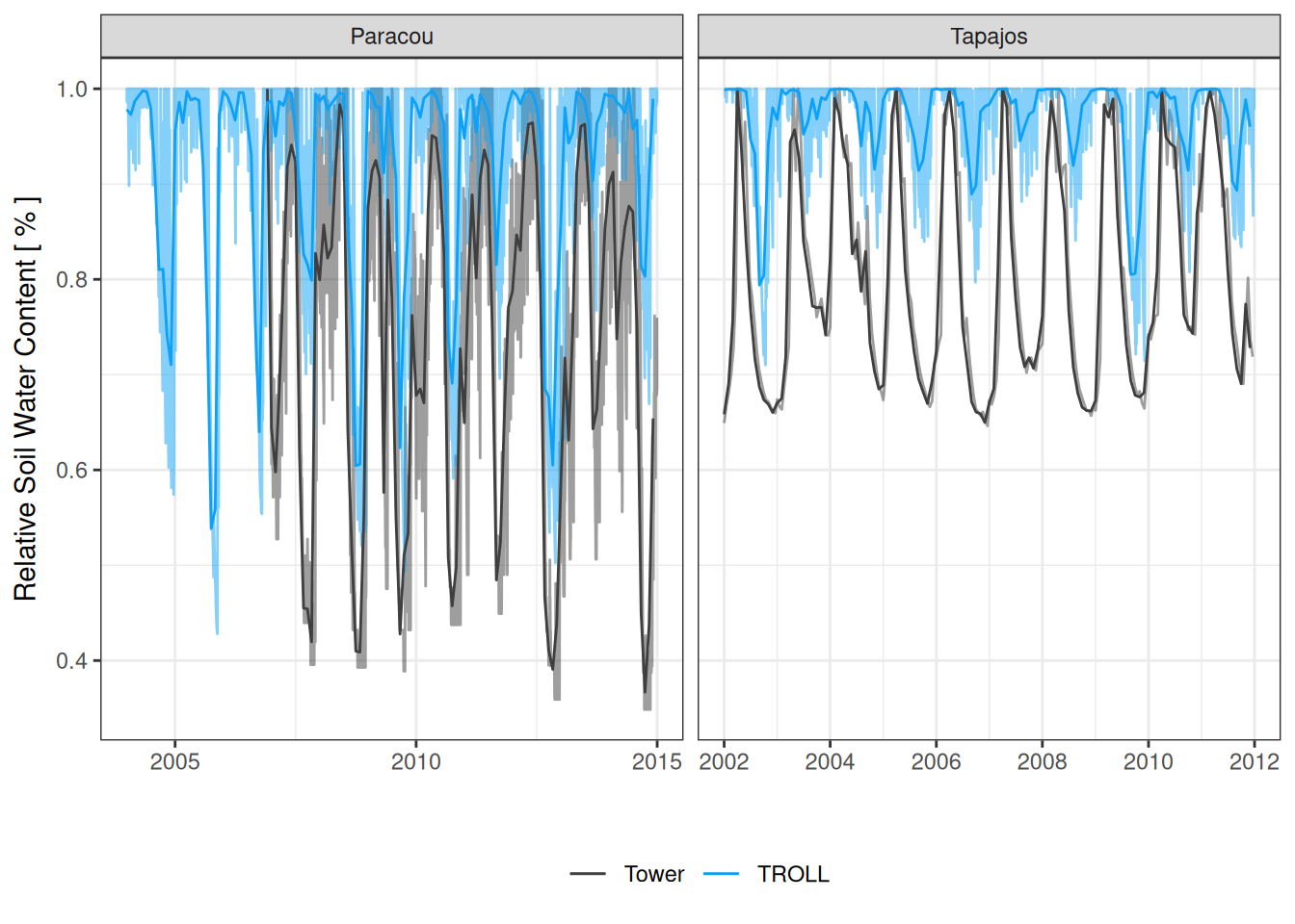
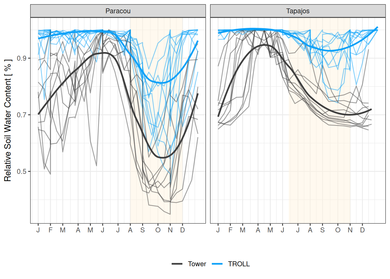
We only had soil water content measurement for Paracou. Moreover, soil water content measurement are measured with electric measurement of conductance and rely a lot on calibration. We thus decided to use Relative Soil water Content (RSWC, %) to avoid bias of tool calibration and focus on within-year variations. The new version of TROLL correctly simulated the phenology of RSWC, with a higher RSWC in wet season around 100% with fully saturated soils and a strong drop in RSWC in the dry season. Focusing on the drop in dry seasons, the mean value simulated across year in Paracou dropped to 80% but exceptionally dry years drop up to 50%. The observed conditions are harsher with a mean observed drop around 50% across years that is below 50 most years and drop to 40% the driest years. Globally, simulated RSWC showed a good evaluation at Paracou with a correlation coefficient of 0.77 against daily observations from eddy-flux towers, and corresponding RMSEP of 23 %.
Daily and monthly means of relative soil water content for Paracou and Tapajos. Dark lines are the monthly means, semi-transparent lines are the daily means variations.
Mean annual cycle from fortnightly means of relative soil water content for Paracou and Tapajos. Bands are the intervals of means across years, and rectangles in the background correspond to the site’s climatological dry season.
Code
daily %>%pivot_wider(names_from = type, values_from = value) %>%na.omit() %>%nest_by(site, variable) %>%mutate(R2 =summary(lm(observed ~0+ simulated, data = data))$r.squared,CC =cor(data$simulated, data$observed),RMSEP =sqrt(mean((data$simulated-data$observed)^2)),RRMSEP =sqrt(mean((data$simulated-data$observed)^2))/mean(data$observed),SD =sd(data$simulated-data$observed),RSD =sd(data$simulated-data$observed)/mean(data$observed)) %>%select(-data) %>% knitr::kable(caption ="Evaluation fo daily means of RSWC at Paracou and Tapajos.")
Evaluation fo daily means of RSWC at Paracou and Tapajos.
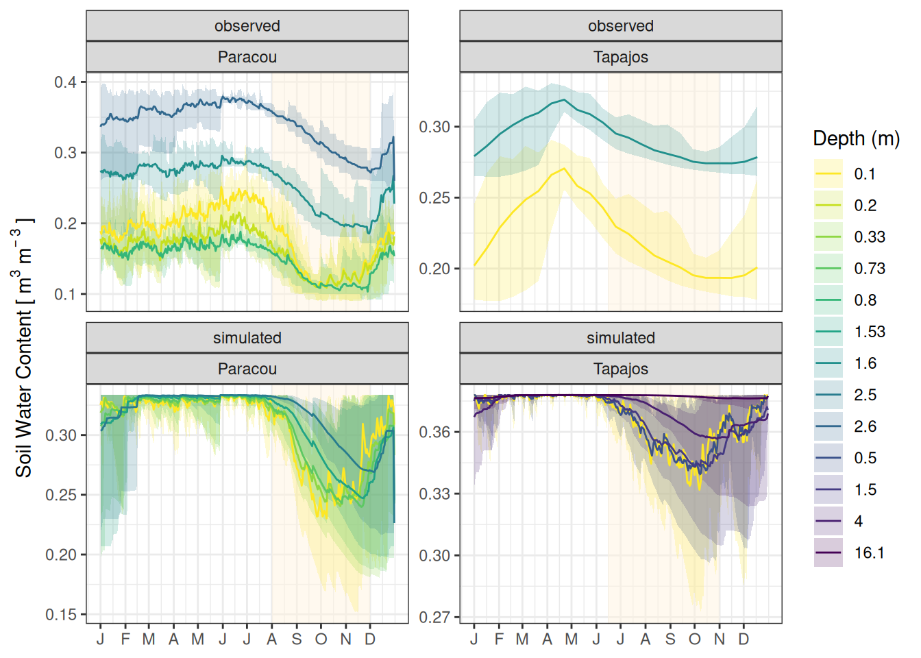
Mean annual cycle from daily means of soil water content for Paracou and Tapajos at different depths. The depth value indicates the maximum depth of the layer. Dark lines are the daily means across years, and bands are the intervals of means across ten years The vertical yellow bands in the background correspond to the site’s climatological dry season.
Yang, Xueqin, Xiuzhi Chen, Jiashun Ren, Wenping Yuan, Liyang Liu, Juxiu Liu, Dexiang Chen, et al. 2023. “A Grid Dataset of Leaf Age-Dependent LAI Seasonality Product (Lad-LAI) over Tropical and Subtropical Evergreen Broadleaved Forests.”http://dx.doi.org/10.5194/essd-2022-436.