Allometric parameters and species functional traits for Paracou and Tapajos were used both as input to the TROLL assessment and as output to assess the functional composition of the forest. Many allometric parameters and functional traits did not exist and were inferred from dbh and height data or by using the relationship between traits with a predictive mean match.
Allometric parameters
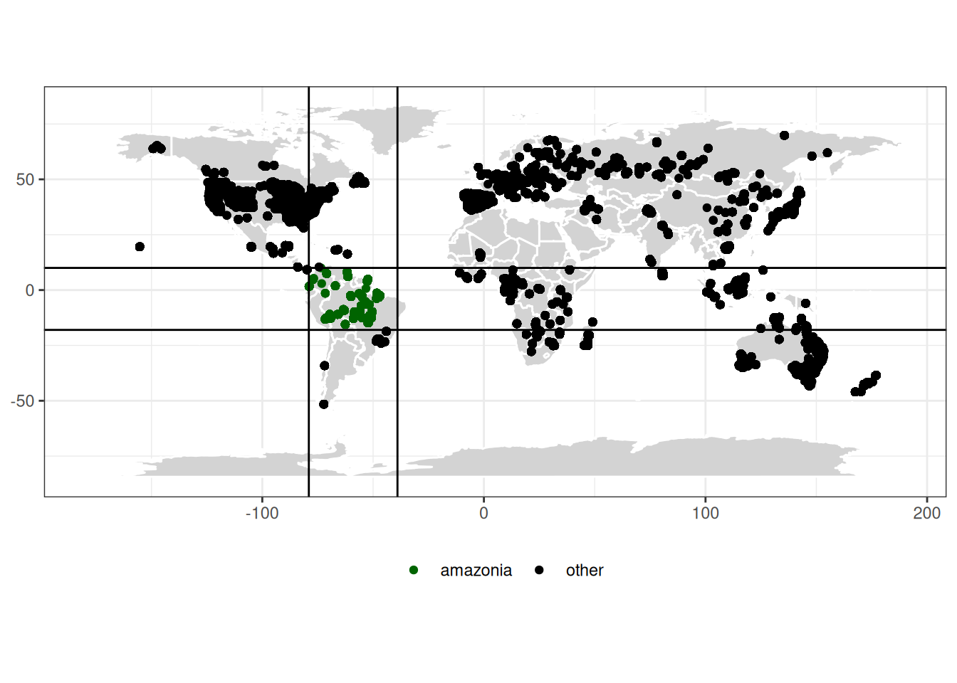
We took advantage of the TALLO database (Jucker et al. 2022) to infer species allometric parameters of the 496 species present in Amazonia (latitude between 10 and -18 and longitude between -78 and -39).
Code
ggplot(map_data("world"), aes(x = long, y = lat)) +geom_polygon(aes(group = group), fill="lightgray", colour ="white") +geom_point(data =read_csv("data/species/tallo.csv") %>%mutate(amazonia =ifelse(longitude <=-39& longitude >=-79& latitude >=-18& latitude <=10, "amazonia", "other")),aes(x = longitude, y = latitude, col = amazonia)) +theme_bw() +geom_hline(yintercept =c(10, -18)) +geom_vline(xintercept =c(-39, -79)) +theme(axis.title =element_blank(), legend.position ="bottom") +scale_color_manual("", values =c("darkgreen", "black")) +coord_equal()
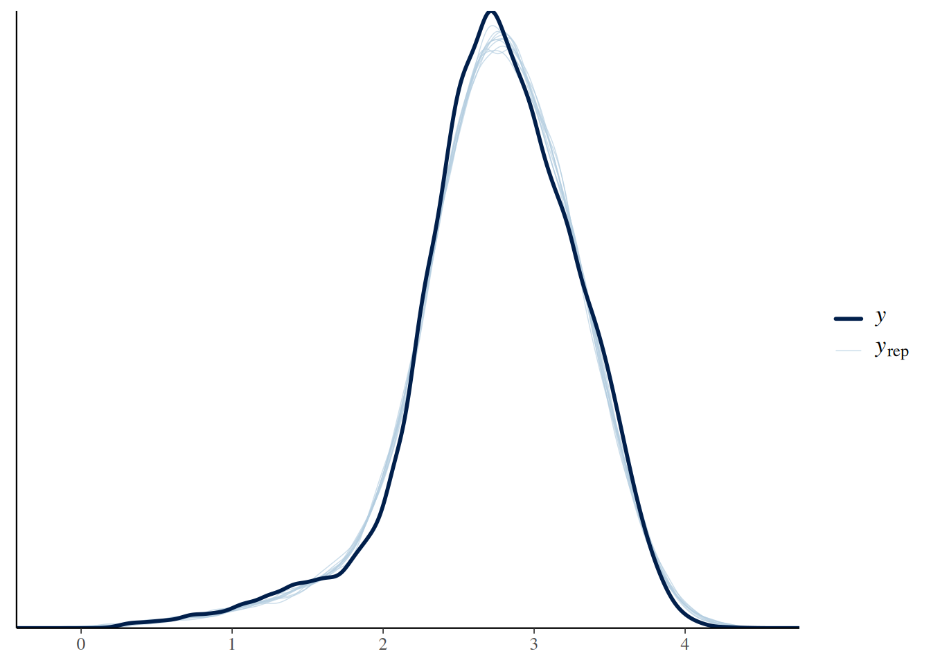
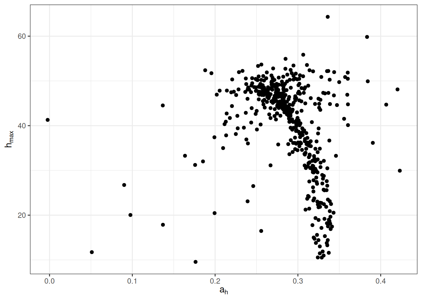
Posterior post-predictive check of simulated response variable against observed values indicating a good representation of the whole distribution in posteriors.
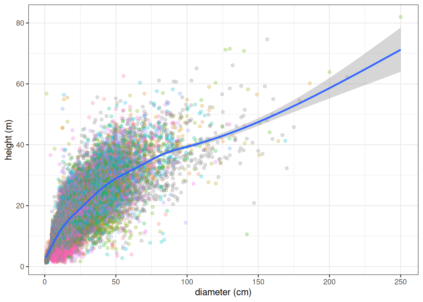
We thus inferred 496 additional \(a_h\), \(h_{max}\) couple of parameters.
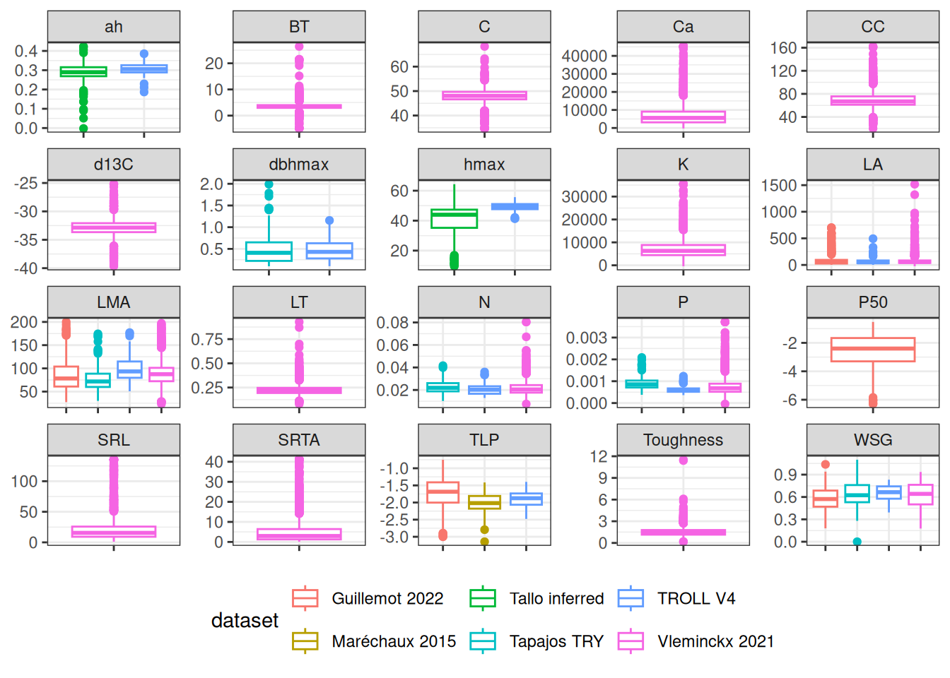
All databases together included 20 traits across 2,921 species but with numerous missing data. Traits distribution were similar across datasets. However, for the same species, allometric parameters inferred from TALLO were lower than those inside TROLL V4 and leaf area from Guillemot was higher than those from TROLL and Vleminckx. As all Paracou TROLL species are in Vleminckx dataset and 109 species from Tapajos we will use only the species from Vleminckx to limit missing data in predictive mean matching (PMM) data imputation.
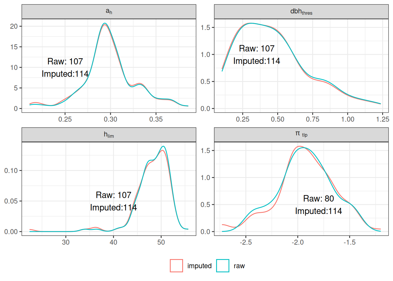
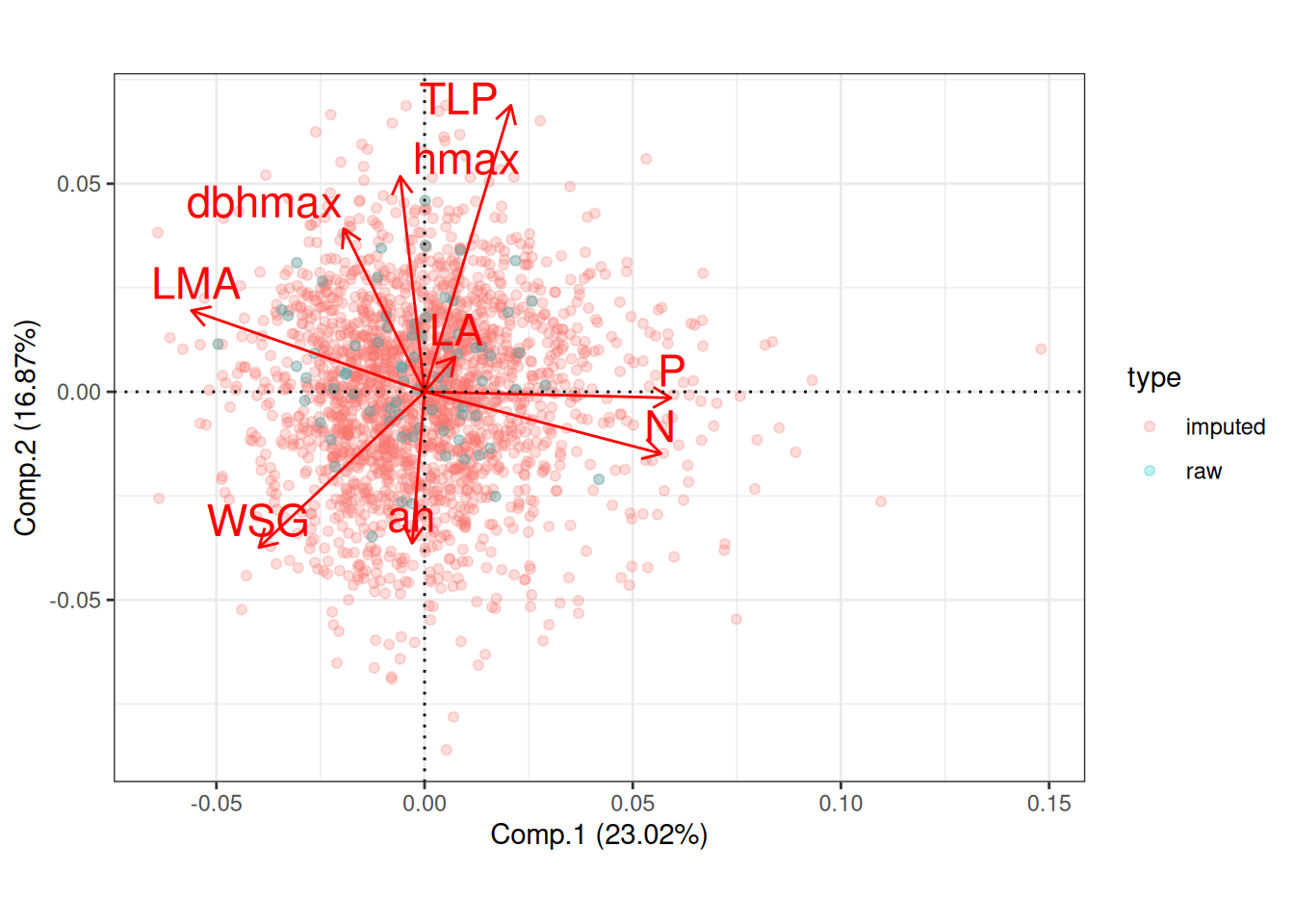
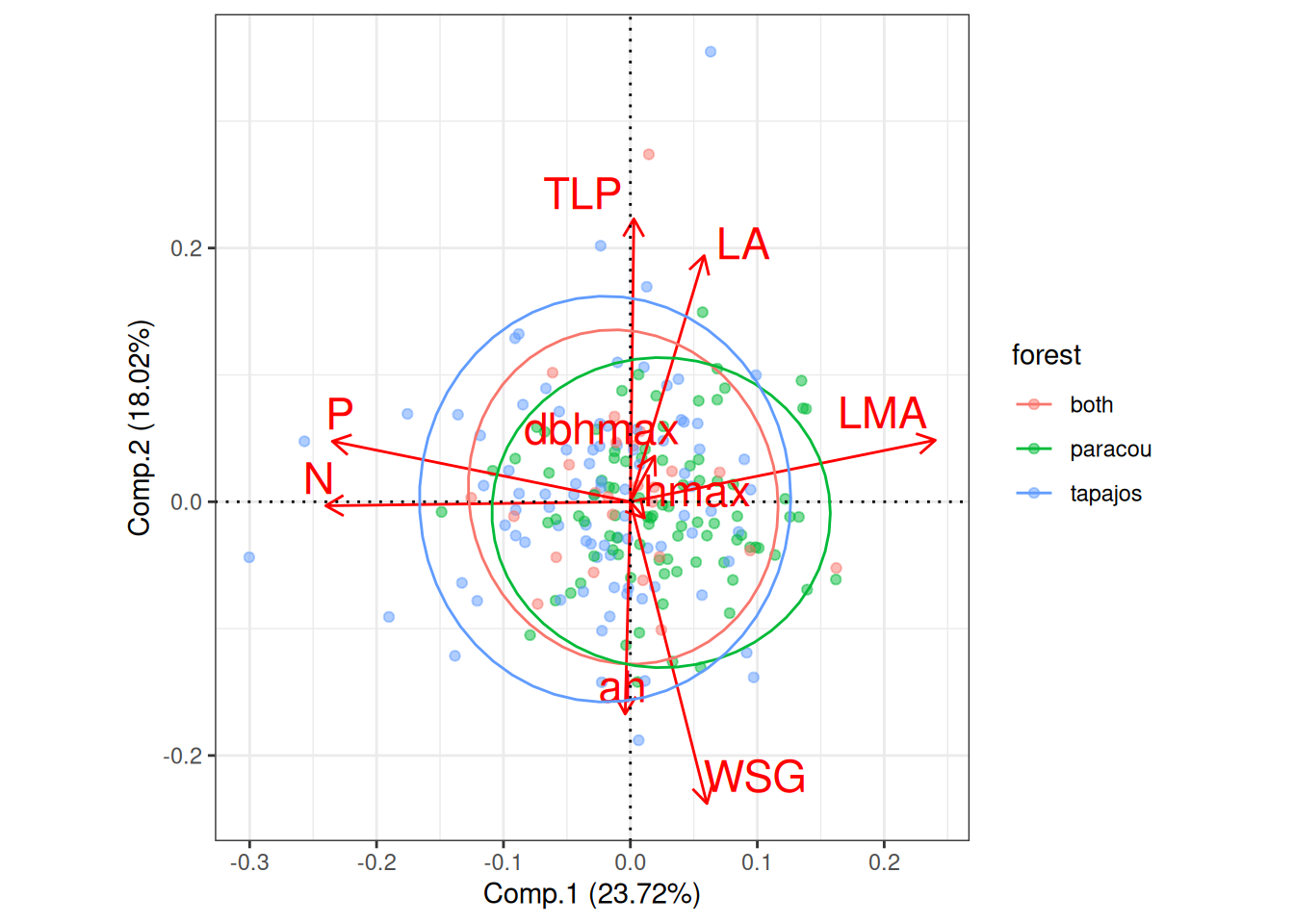
Missing data were too important to use random forest for imputation with missForest even with phylogenetic eigen values. Thus, we used simple predictive mean matching (PMM) data imputation with mice without phylogenetic eigen values. However, phylogenetic eigen values could also been used with phylomice (not done here). As we focused on species in common with Vlemincks data we only had to impute ah, dbhmax, hmax and TLP with values from Maréchaux, Tapajos and inferred with TALLO. Obtained imputed distributions matched well the observed distribution of the raw data and imputed functional space match the one of the raw data (PCA). The PCA also revealed similar functional spaces between species from Paracou and Tapajos, whereas Tapajos functional space is a bit wider.
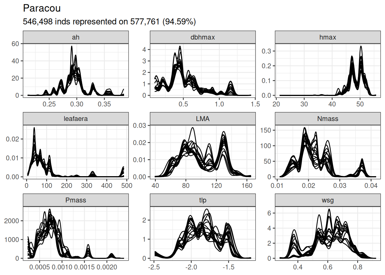
Forest functional composition was simply assessed using functional trait distribution in each plots (repeted lines in Paracou data) at the species level in Paracou and genus level in Tapajos.
Functional composition at the Paracou site expressed in terms of density distribution per trait. The analyses have been done at the species level in Paracou.
Code
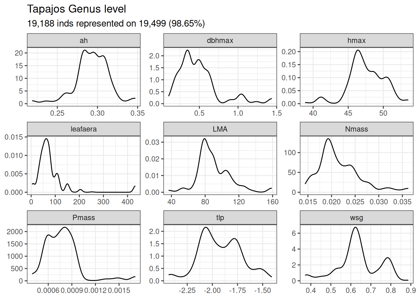
read_tsv("outputs/functional_composition.tsv") %>%filter(site =="Tapajos") %>%ggplot(aes(trait_value, group = plot)) +geom_density() +facet_wrap(~ trait, scales ="free") +theme_bw() +ggtitle("Tapajos Genus level", "19,188 inds represented on 19,499 (98.65%)") +theme(axis.title =element_blank(), legend.position ="bottom") +scale_color_discrete("")
Functional composition at the Tapajos site expressed in terms of density distribution per trait. The analyses have been done at the genus level in Tapajos.
Baraloto, Christopher, C. E. Timothy Paine, Sandra Patiño, Damien Bonal, Bruno Hérault, and Jerome Chave. 2010. “Functional Trait Variation and Sampling Strategies in Species-Rich Plant Communities.”Functional Ecology 24 (1): 208–16. https://doi.org/10.1111/j.1365-2435.2009.01600.x.
Guillemot, Joannès, Nicolas K. Martin-StPaul, Leticia Bulascoschi, Lourens Poorter, Xavier Morin, Bruno X. Pinho, Guerric le Maire, et al. 2022. “Small and Slow Is Safe: On the Drought Tolerance of Tropical Tree Species.”Global Change Biology 28 (8): 2622–38. https://doi.org/10.1111/gcb.16082.
Jucker, Tommaso, Fabian Jörg Fischer, Jérôme Chave, David A. Coomes, John Caspersen, Arshad Ali, Grace Jopaul Loubota Panzou, et al. 2022. “Tallo: A Global Tree Allometry and Crown Architecture Database.”Global Change Biology 28 (17): 5254–68. https://doi.org/10.1111/gcb.16302.
Kattge, Jens, Gerhard Bönisch, and et al. 2020. “TRY Plant Trait Database – Enhanced Coverage and Open Access.”Global Change Biology 26: 119–88. https://doi.org/10.1111/gcb.14904.
Maréchaux, Isabelle, Megan K. Bartlett, Lawren Sack, Christopher Baraloto, Julien Engel, Emilie Joetzjer, and Jérôme Chave. 2015. “Drought Tolerance as Predicted by Leaf Water Potential at Turgor Loss Point Varies Strongly Across Species Within an Amazonian Forest.” Edited by Kaoru Kitajima. Functional Ecology 29 (10): 1268–77. https://doi.org/10.1111/1365-2435.12452.
Maréchaux, Isabelle, and Jérôme Chave. 2017. “An Individual-Based Forest Model to Jointly Simulate Carbon and Tree Diversity in Amazonia: Description and Applications.”Ecological Monographs 87 (4): 632–64. https://doi.org/10.1002/ecm.1271.
Maréchaux, Isabelle, Laurent Saint-André, Megan K. Bartlett, Lawren Sack, and Jérôme Chave. 2019. “Leaf Drought Tolerance Cannot Be Inferred from Classic Leaf Traits in a Tropical Rainforest.” Edited by Pierre Mariotte. Journal of Ecology 108 (3): 1030–45. https://doi.org/10.1111/1365-2745.13321.
Schmitt, Sylvain, and Marion Boisseaux. 2023. “Higher Local Intra- Than Interspecific Variability in Water- and Carbon-Related Leaf Traits Among Neotropical Tree Species.”Annals of Botany 131 (5): 801–11. https://doi.org/10.1093/aob/mcad042.
Vleminckx, Jason, Claire Fortunel, Oscar Valverde-Barrantes, C. E. Timothy Paine, Julien Engel, Pascal Petronelli, Aurélie K. Dourdain, Juan Guevara, Solène Béroujon, and Christopher Baraloto. 2021. “Resolving Whole-Plant Economics from Leaf, Stem and Root Traits of 1467 Amazonian Tree Species.”Oikos 130 (7): 1193–1208. https://doi.org/10.1111/oik.08284.
Ziegler, Camille, Sabrina Coste, Clément Stahl, Sylvain Delzon, Sébastien Levionnois, Jocelyn Cazal, Hervé Cochard, et al. 2019. “Large Hydraulic Safety Margins Protect Neotropical Canopy Rainforest Tree Species Against Hydraulic Failure During Drought.”Annals of Forest Science 76 (4). https://doi.org/10.1007/s13595-019-0905-0.