Phenology

Calibration of the new leaf phenology modules against observed litterfall in Paracou and Tapajos. Parameters include:

• a: the leaf resistance parameter
• b: the tree height susceptibility parameter
• delta: the base variation in residence time multiplying factor for drought shedding

Code

prep_sim <- function(f) {
  t <- vroom::vroom(f)  %>% 
    select(iter, litterfall) %>% 
    mutate(file = f) %>% 
    mutate(file = gsub("results/calib_pheno/", "", file)) %>% 
    mutate(file = gsub("_0_sumstats.txt", "", file)) %>% 
    separate(file, c("site", "a0", "b0", "delta"), "_", convert = T) %>% 
    mutate(date = as_date(ifelse(site == "Tapajos", 
                                 "2002/01/01", "2004/01/01")) + iter) %>% 
    mutate(litterfall = litterfall*365) %>% 
    select(-iter) %>% 
    left_join(vroom::vroom("outputs/litter.tsv") %>% 
                rename(observed = litterfall))
  t$obs_group <- NA
  t$obs_group[!is.na(t$dt)] <- 1:length(t$dt[!is.na(t$dt)])
  t %>% 
    fill(obs_group, .direction = "up") %>% 
    mutate(dt_full = dt) %>% 
    fill(dt_full, .direction = "up") %>% 
    group_by(obs_group) %>% 
    filter(n() >= dt_full) %>% 
    mutate(simulated = ifelse(!is.na(dt), 
                              zoo::rollmeanr(litterfall, unique(dt_full), fill = NA), 
                              NA)) %>% 
    ungroup() %>% 
    select(site, a0, b0, delta, date, dt, observed, simulated) %>% 
    na.omit()
}

files <- list.files("results/calib_pheno", full.names = T, pattern = "sumstats.txt")
names(files) <- list.files("results/calib_pheno", full.names = F, pattern = "sumstats.txt")
raw <- files %>% 
  lapply(prep_sim)  %>% 
  bind_rows()
write_tsv(raw, "outputs/calib.tsv")

Code

prep_sim <- function(f) {
  t <- vroom::vroom(f)  %>% 
    select(iter, litterfall) %>% 
    mutate(iter = iter - 219000 + 365*10 + 1) %>% 
    filter(iter > 0) %>% 
    mutate(file = f) %>% 
    mutate(file = gsub("results/test_ll_isa/", "", file)) %>% 
    mutate(file = gsub("_testLL_0_sumstats.txt", "", file)) %>% 
    mutate(file = gsub("TROLLv4_", "", file)) %>% 
    rename(site = file) %>% 
    mutate(date = as_date(ifelse(site == "Tapajos", 
                                 "2002/01/01", "2004/01/01")) + iter) %>% 
    mutate(litterfall = litterfall*365) %>% 
    select(-iter) %>% 
    left_join(vroom::vroom("outputs/litter.tsv") %>% 
                rename(observed = litterfall))
  t$obs_group <- NA
  t$obs_group[!is.na(t$dt)] <- 1:length(t$dt[!is.na(t$dt)])
  t %>% 
    fill(obs_group, .direction = "up") %>% 
    mutate(dt_full = dt) %>% 
    fill(dt_full, .direction = "up") %>% 
    group_by(obs_group) %>% 
    filter(n() >= dt_full) %>% 
    mutate(simulated = ifelse(!is.na(dt), 
                              zoo::rollmeanr(litterfall, unique(dt_full), fill = NA), 
                              NA)) %>% 
    ungroup() %>% 
    select(site, date, dt, observed, simulated) %>% 
    na.omit()
}

files <- list.files("results/test_ll_isa", full.names = T, pattern = "sumstats.txt")
names(files) <- list.files("results/test_ll_isa", full.names = F, pattern = "sumstats.txt")
raw <- files %>% 
  lapply(prep_sim)  %>% 
  bind_rows()
write_tsv(raw, "outputs/calib_test_ll_isa.tsv")

Code

sim_metrics <- read_tsv("outputs/calib.tsv") %>% 
  gather(type, litterfall, -site, -a0, -b0, -delta, -date, -dt) %>% 
  group_by(site, a0, b0, delta, year = year(date), type) %>% 
    summarise(peak = mean(c(litterfall[which.max(litterfall)],
                          litterfall[which.max(litterfall)-1],
                          litterfall[which.max(litterfall)+1]), na.rm = TRUE),
            peak_date = date[which.max(litterfall)],
            basal = mean(as.numeric(month(date) %in% 1:4)*litterfall, na.rm = TRUE)) %>%  
  mutate(peak_day = yday(peak_date), ratio = peak / basal) %>% 
  filter(basal > 0, peak_day > 100)

Parameters effect

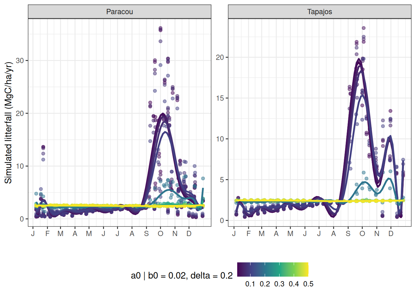
The leaf resistance parameter which is limiting the potential at turgor loss point (TLP, see methods) is manly limiting the height of litterfall peak in dry season with a peak up to 30 MgC/ha/yr with a at 0.01 against no peak with high values above 0.3. An higher leaf resistance above 0.1 also results in a latter peak. Globally, the less resistant are the leaves of the trees the higher is the litterfall in dry conditions.

Code

ga1 <- read_tsv("outputs/calib.tsv") %>% 
  filter(b0 == 0.02, delta == 0.2) %>% 
  ggplot(aes(yday(date), simulated, col = a0, fill = a0)) +
  geom_point(alpha = 0.5) +
  geom_smooth(aes(group = as.factor(a0)), method = "lm", se = FALSE, 
              formula = y ~ poly(x, 20, raw = TRUE)) +
  theme_bw() +
  facet_wrap(~ site, scales = "free", nrow = 1) +
  scale_color_viridis_c("Year") +
  xlab("") + ylab("Simulated litterfall (MgC/ha/yr)") +
  scale_x_continuous(breaks = yday(as_date(paste0("2001-", 1:12, "-1"))),
                   labels = c("J", "F", "M", "A", "M", "J", "J", "A", "S", "O", "N", "D")) +
  scale_color_viridis_c("a0 | b0 = 0.02, delta = 0.2") +
  scale_fill_viridis_c("a0 | b0 = 0.02, delta = 0.2") +
  theme(legend.position = "bottom")
ga1

Effect of the leaf resistance parameter a on the annual cycle from fortnightly litterfall for Paracou and Tapajos.

Code

ga2 <- sim_metrics %>% 
  filter(b0 == 0.02, delta == 0.2, type == "simulated") %>% 
  ggplot(aes(peak_day, ratio, col = a0)) +
  geom_point() +
  theme_bw() +
  facet_wrap(~ site) +
  ylab("Simulated litterfall ratio") +
  xlab("Simulated litterfall peak day") +
  scale_color_viridis_c() +
  scale_color_viridis_c("a0 | b0 = 0.02, delta = 0.2") +
  theme(legend.position = "bottom")
ga2

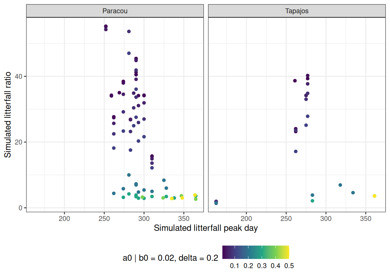
Effect of the leaf resistance parameter a on the relation between Litterfall peak date and ratioi across years at Paracou and Tapajos.

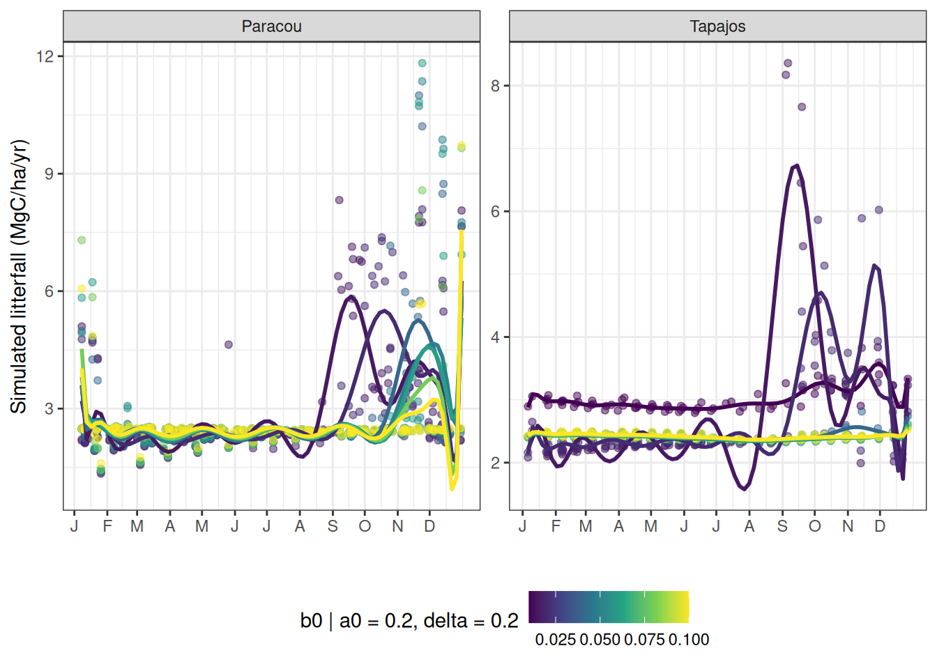
The the tree height susceptibility parameter drives mainly the peak date but also the peak intensity for values above 0.1. Indeed low values close to 0.01 show a peak starting in September, whereas high values have a peak starting in December.

Code

gb1 <- read_tsv("outputs/calib.tsv") %>% 
  filter(a0 == 0.2, delta == 0.2) %>% 
  ggplot(aes(yday(date), simulated, col = b0, fill = b0)) +
  geom_point(alpha = 0.5) +
  geom_smooth(aes(group = as.factor(b0)), method = "lm", se = FALSE, 
              formula = y ~ poly(x, 20, raw = TRUE)) +
  theme_bw() +
  facet_wrap(~ site, scales = "free", nrow = 1) +
  scale_color_viridis_c("Year") +
  xlab("") + ylab("Simulated litterfall (MgC/ha/yr)") +
  scale_x_continuous(breaks = yday(as_date(paste0("2001-", 1:12, "-1"))),
                   labels = c("J", "F", "M", "A", "M", "J", "J", "A", "S", "O", "N", "D")) +
  scale_color_viridis_c("b0 | a0 = 0.2, delta = 0.2") +
  scale_fill_viridis_c("b0 | a0 = 0.2, delta = 0.2") +
  theme(legend.position = "bottom")
gb1

Effect of the tree height susceptibility parameter b on the annual cycle from fortnightly litterfall for Paracou and Tapajos.

Code

gb2 <- sim_metrics %>% 
  filter(a0 == 0.2, delta == 0.2, type == "simulated") %>% 
  ggplot(aes(peak_day, ratio, col = b0)) +
  geom_point() +
  theme_bw() +
  facet_wrap(~ site) +
  ylab("Simulated litterfall ratio") +
  xlab("Simulated litterfall peak day") +
  scale_color_viridis_c() +
  scale_color_viridis_c("b0 | a0 = 0.2, delta = 0.2") +
  theme(legend.position = "bottom")
gb2

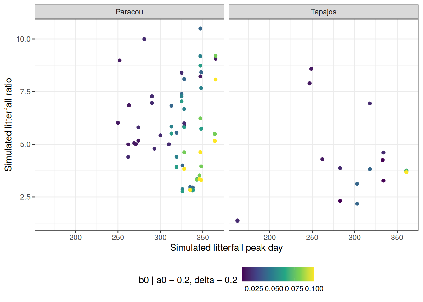
Effect of the tree height susceptibility parameter b on the relation between Litterfall peak date and ratioi across years at Paracou and Tapajos.

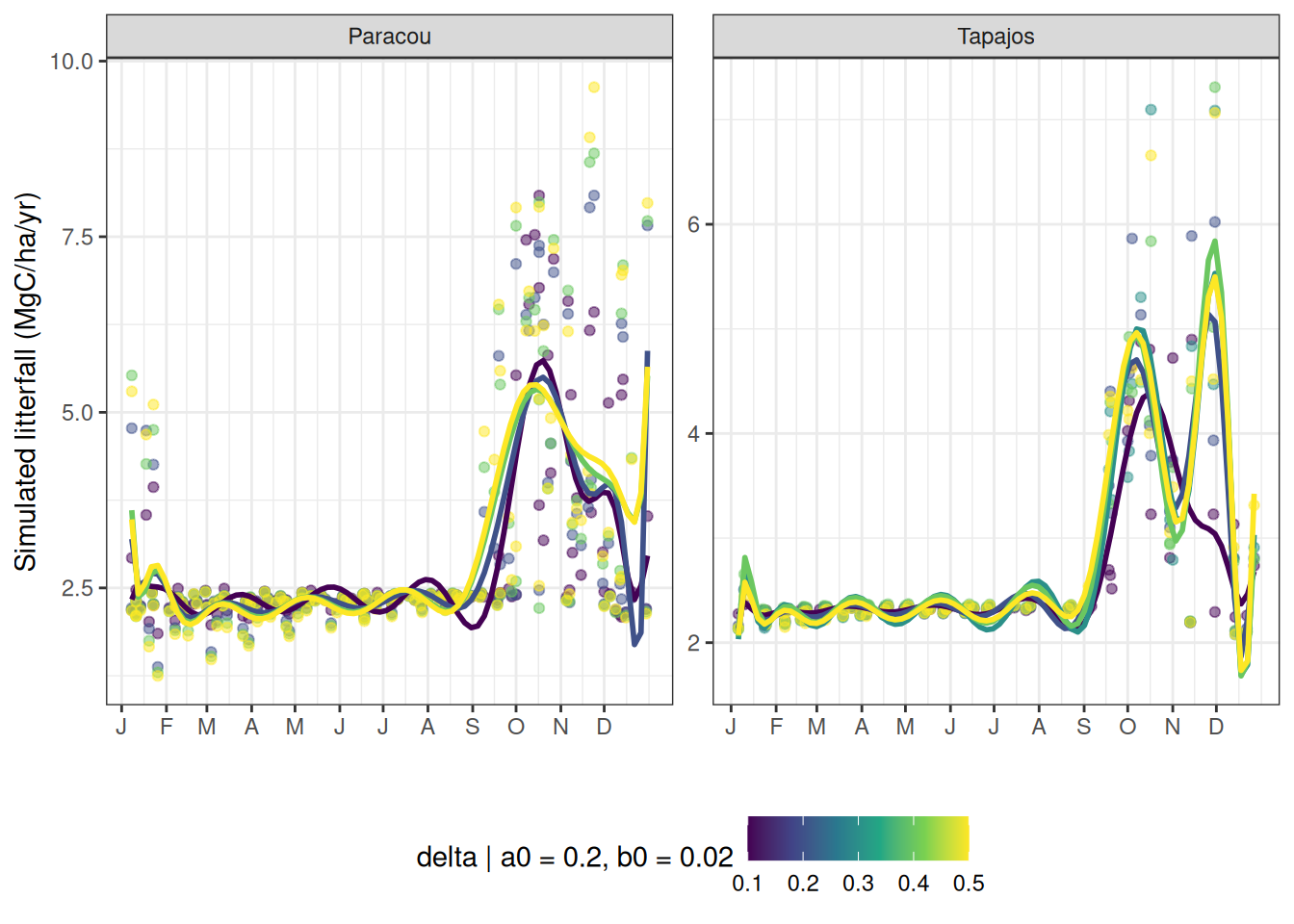
The base variation in residence time multiplying factor for drought shedding seems to have a lighter influence on litterfall peak intensity and date, at least for default values of the two other parameters.

Code

gd1 <- read_tsv("outputs/calib.tsv") %>% 
  filter(b0 == 0.02, a0 == 0.2) %>% 
  ggplot(aes(yday(date), simulated, col = delta, fill = delta)) +
  geom_point(alpha = 0.5) +
  geom_smooth(aes(group = as.factor(delta)), method = "lm", se = FALSE, 
              formula = y ~ poly(x, 20, raw = TRUE)) +
  theme_bw() +
  facet_wrap(~ site, scales = "free", nrow = 1) +
  scale_color_viridis_c("Year") +
  xlab("") + ylab("Simulated litterfall (MgC/ha/yr)") +
  scale_x_continuous(breaks = yday(as_date(paste0("2001-", 1:12, "-1"))),
                   labels = c("J", "F", "M", "A", "M", "J", "J", "A", "S", "O", "N", "D")) +
  scale_color_viridis_c("delta | a0 = 0.2, b0 = 0.02") +
  scale_fill_viridis_c("delta | a0 = 0.2, b0 = 0.02") +
  theme(legend.position = "bottom")
gd1

Effect of the base variation in residence time multiplying factor for drought shedding delta on the annual cycle from fortnightly litterfall for Paracou and Tapajos.

Code

gd2 <- sim_metrics %>% 
  filter(b0 == 0.02, a0 == 0.2, type == "simulated") %>% 
  ggplot(aes(peak_day, ratio, col = delta)) +
  geom_point() +
  theme_bw() +
  facet_wrap(~ site) +
  ylab("Simulated litterfall ratio") +
  xlab("Simulated litterfall peak day") +
  scale_color_viridis_c() +
  scale_color_viridis_c("delta | a0 = 0.2, b0 = 0.02") +
  theme(legend.position = "bottom")
gd2

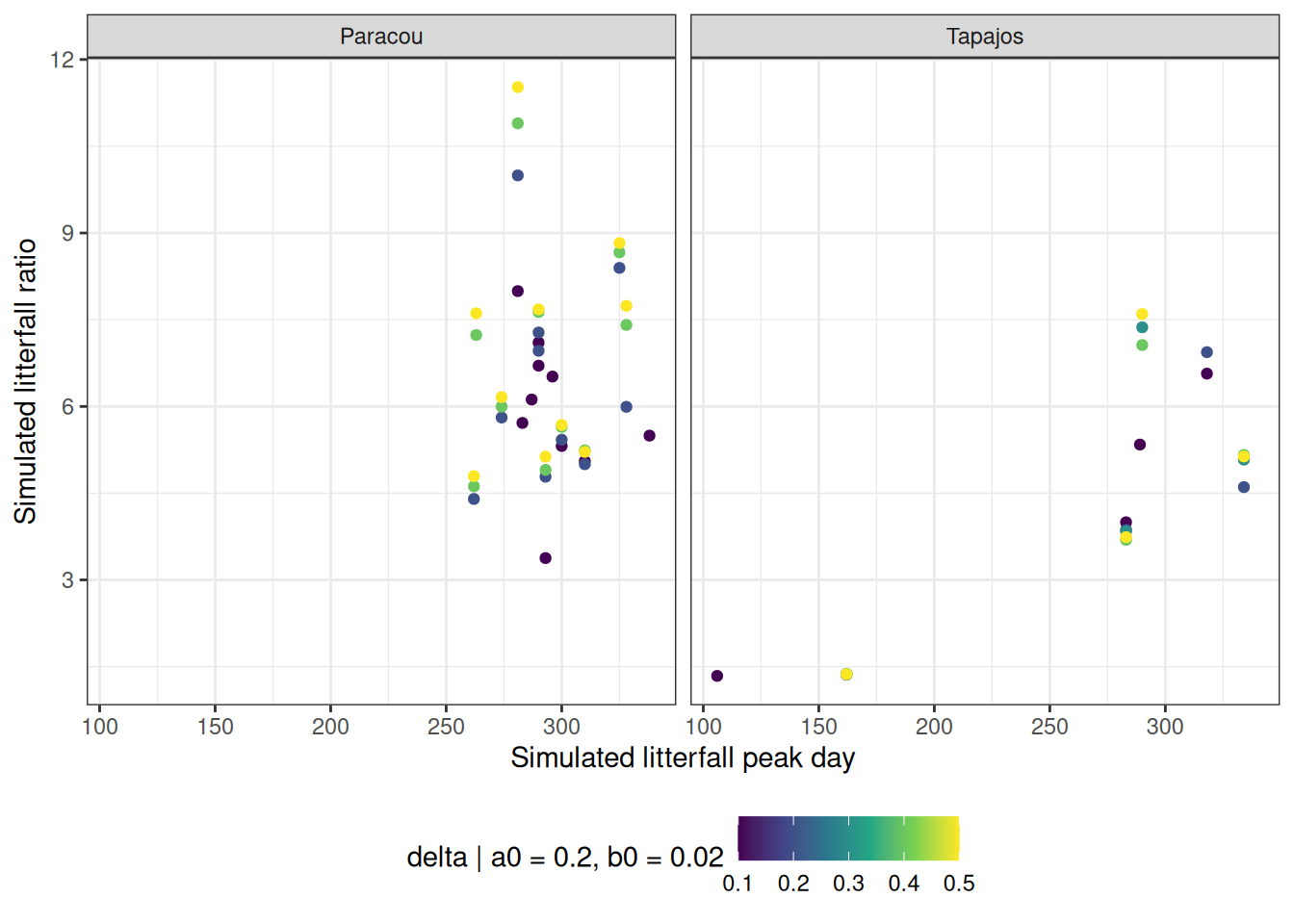
Effect of the base variation in residence time multiplying factor for drought shedding delta on the relation between Litterfall peak date and ratioi across years at Paracou and Tapajos.

Code

g <- cowplot::plot_grid(ga1 + 
                          ggtitle("a0 | b0 = 0.02, delta = 0.2") +
                          theme(legend.position = "none"), 
                        gb1+ 
                          ggtitle("b0 | a0 = 0.2, delta = 0.2") +
                          theme(legend.position = "none"), 
                        gd1+ 
                          ggtitle("delta | a0 = 0.2, b0 = 0.02") +
                          theme(legend.position = "none"), 
                        ga2 +
                          scale_color_viridis_c(""),
                        gb2 +
                          scale_color_viridis_c(""), 
                        gd2 +
                          scale_color_viridis_c(""),
                        nrow = 2)
ggsave("figures/fa05.png", g, dpi = 300, width = 16, height = 8, bg = "white")

Sensitivity to parameters

Code

calib_str1 <- read_tsv("outputs/calib_str4.tsv") %>% 
  group_by(site, a, b, m) %>% 
  summarise(abundance = sum(abundance), agb = sum(agb), ba = sum(ba))
sens_str1 <- lapply(c("abundance", "agb", "ba"), function(var) 
  sensitivity::pcc(calib_str1[c("a", "b", "m")], 
                   calib_str1[var], 
                   nboot = 100)$PCC %>%
    rownames_to_column(var = "parameter") %>% 
    mutate(variable = var)) %>% 
  bind_rows()
calib_pheno <- sim_metrics %>% filter(type == "simulated")
sens_pheno <- lapply(c("peak_day", "ratio"), function(var) 
  sensitivity::pcc(calib_pheno[c("a0", "b0", "delta")], 
                   calib_pheno[var], 
                   nboot = 100)$PCC %>%
    rownames_to_column(var = "parameter") %>% 
    mutate(variable = var)) %>% 
  bind_rows()
calib_str2 <- data.frame(file = list.files("results/calib_pheno/")) %>% 
  rowwise() %>% 
  mutate(structure = list(read_tsv(file.path("results", "calib_pheno", file),
                                   col_select = c(3,5,7), skip = 4015, col_names = F) %>% 
                            tail(1))) %>% 
  unnest(structure) %>% 
  rename(abundance = X3, ba = X5, agb = X7) %>% 
  separate(file, c("site", "a0", "b0", "delta"), sep = "_", convert = TRUE)
sens_str2 <- lapply(c("abundance", "ba", "agb"), function(var) 
  sensitivity::pcc(calib_str2[c("a0", "b0", "delta")], 
                   calib_str2[var], 
                   nboot = 100)$PCC %>%
    rownames_to_column(var = "parameter") %>% 
    mutate(variable = var)) %>% 
  bind_rows()
bind_rows(sens_str1, sens_pheno, sens_str2) %>% 
  write_tsv("outputs/sensitivity.tsv")

Code

g <- read_tsv("outputs/sensitivity.tsv") %>% 
   mutate(type = ifelse(parameter %in% c("a", "b", "m"),
                        "Structure", "Litterfall")) %>% 
  mutate(type = factor(type, levels = c("Structure", "Litterfall"))) %>% 
    mutate(parameter = recode(parameter,
                              "a" = "a[CR]",
                              "b" = "b[CR]",
                              "m" = "m",
                              "a0" = "a[0]",
                              "b0" = "b[0]",
                              "delta" = "delta[0]")) %>% 
   mutate(variable = recode(variable,
                            "abundance" = "Number of stems",
                            "agb" = "Aboveground biomass",
                            "ba" = "Basal area",
                            "peak_day" = "Litterfall peak day",
                            "ratio" = "Litterfall peak ratio")) %>% 
  ggplot(aes(parameter, original, 
             ymin = `min. c.i.`, ymax = `max. c.i.`, 
             fill = variable)) + 
  geom_col(position = position_dodge2(width = 0.9, preserve = "single")) + 
  geom_linerange(position = position_dodge2(width = 0.9, preserve = "single"),
                 colour = "black") +
  theme_bw() +
  ylab("Partial Correlation Coefficients (PCC)") + xlab("") +
  theme(legend.position = "bottom") +
  scale_x_discrete(labels = scales::label_parse()) +
  scale_fill_discrete("") +
  facet_wrap(~ type, scales = "free_x")
ggsave("figures/fa04.png", g, dpi = 300, width = 8, height = 6, bg = "white")

Code

g <- read_tsv("outputs/calib_str4.tsv") %>% 
  select(-dbh_class) %>% 
  group_by(site, a, b, m) %>% 
  summarise_all(sum) %>% 
  mutate(agb  = agb/10^3) %>% 
  ungroup() %>% 
  filter(ba > 10) %>% 
  gather(variable, value, -site, -a, -b, -m) %>% 
  gather(parameter, par_value, -site, -variable, -value) %>%
  group_by(parameter) %>% 
  mutate(par_value = scale(par_value)) %>% 
  mutate(parameter = recode(parameter,
                              "a" = "a[CR]",
                              "b" = "b[CR]",
                              "m" = "m")) %>% 
   mutate(variable = recode(variable,
                            "abundance" = "N",
                            "agb" = "AGB",
                            "ba" = "BA")) %>% 
    ggplot(aes(par_value, value)) +
    geom_point(alpha = .1) +
    facet_grid(variable ~ parameter, scales = "free", labeller = label_parsed) +
    theme_bw() +
    geom_smooth(method = "lm") +
  ggpubr::stat_regline_equation(col = "blue") +
  xlab("Standard value") + ylab("")
ggsave("figures/fa13.png", g, dpi = 300, width = 8, height = 6, bg = "white")

Best parameters

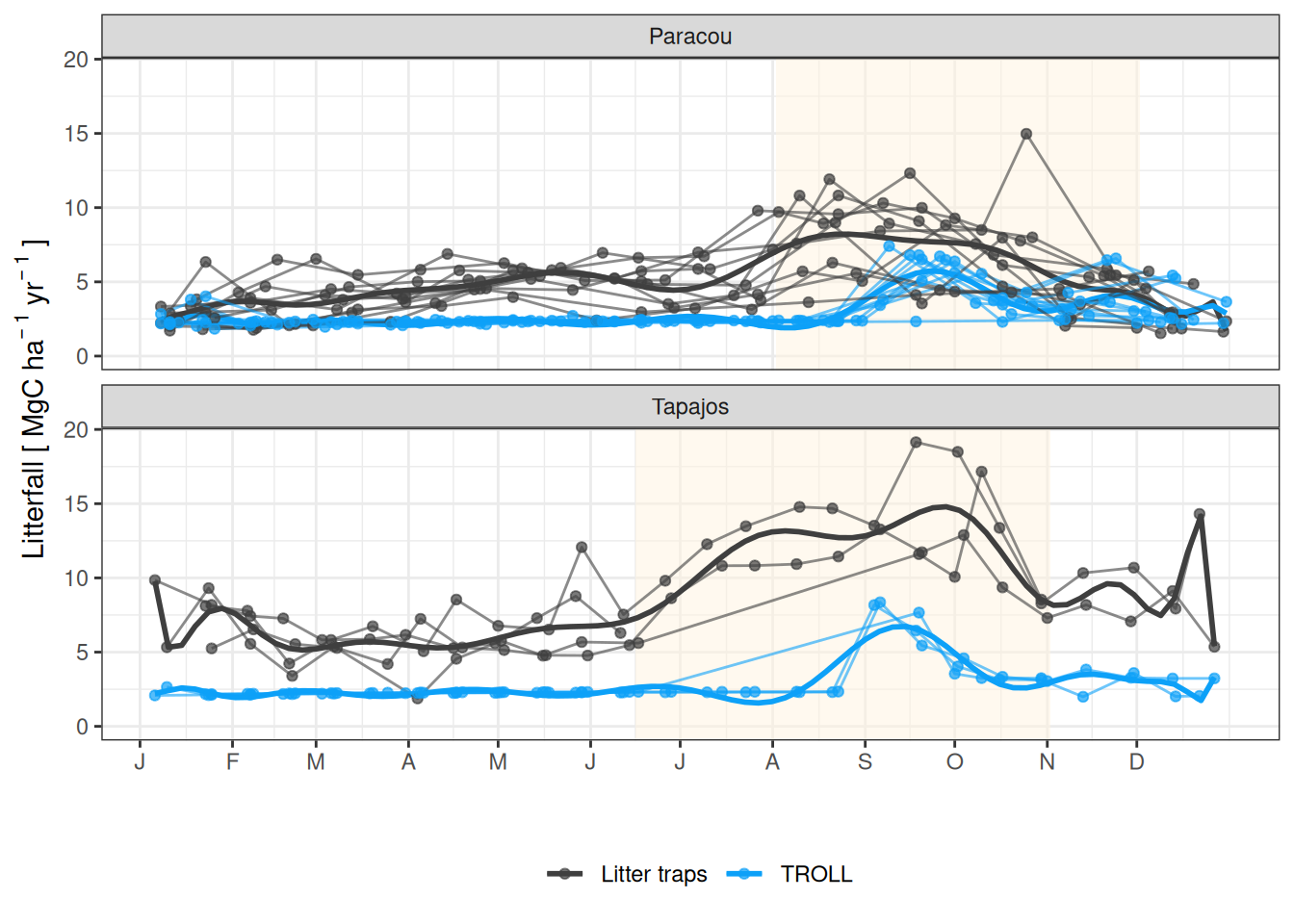
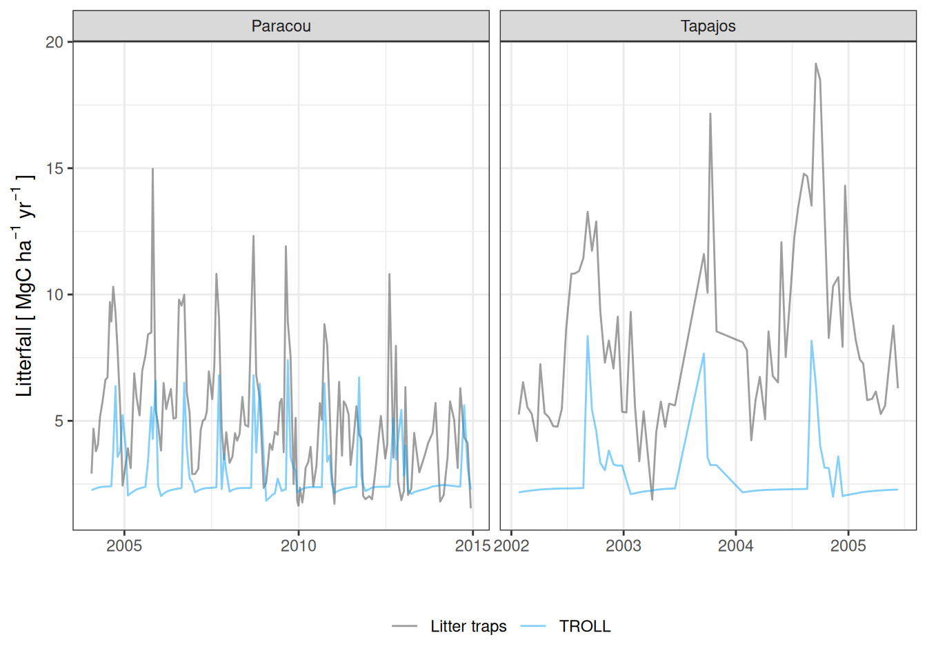
We found similar \(a=0.2\) and \(b=0.015\) to be the best in Paracou and Tapajos, but slightly different \(delta\) with \(delta=0.1\) in Paracou and \(delta=0.2\) in Tapajos. Except for delta in Tapajos all values are outside the limit of parameters explorations. The resulting litterfall dynamics of the simulations follows the intrannual pattern of observed litterfall with an early dry season peak (~September Paracou, ~August Tapajos) of around 7 times the basal flux observed in the wet season. However, the model still have issues to simulated the intensity of the basal flux, especially in Tapajos.

Code

sim_metrics %>% 
  ungroup() %>% 
  mutate(ratio = as.vector(scale(ratio)), 
         peak_day = as.vector(scale(peak_day))) %>% 
  gather(metric, value, -site, -a0, -b0, -delta, -year, -type) %>% 
  filter(metric %in% c("ratio", "peak_day")) %>% 
  mutate(metric = paste0(metric, "_", type)) %>% 
  select(-type) %>% 
  pivot_wider(names_from = metric, values_from = value) %>% 
  na.omit() %>% 
  mutate(
    error_both = sqrt((ratio_observed - ratio_simulated)^2
                      +(peak_day_observed - peak_day_simulated)^2),
    error_peak = sqrt((peak_day_observed - peak_day_simulated)^2),
    error_ratio = sqrt((ratio_observed - ratio_simulated)^2),
    ) %>% 
  group_by(site, a0, b0, delta) %>% 
  summarise(both = sqrt(mean(error_both^2, na.rm = T)),
            peak = sqrt(mean(error_peak^2, na.rm = T)),
            ratio = sqrt(mean(error_ratio^2, na.rm = T))) %>% 
  gather(metric, rmsep, -site, -a0, -b0, -delta, -site) %>%  
  group_by(site, metric) %>% 
  slice_min(rmsep) %>% 
  knitr::kable()

site	a0	b0	delta	metric	rmsep
Paracou	0.200	0.015	0.1	both	1.0616194
Paracou	0.075	0.015	0.4	peak	0.6097572
Paracou	0.100	0.015	0.4	peak	0.6097572
Paracou	0.200	0.015	0.3	ratio	0.1707245
Tapajos	0.200	0.015	0.2	both	0.3327142
Tapajos	0.300	0.015	0.2	peak	0.0000000
Tapajos	0.100	0.050	0.4	ratio	0.0644877

Code

sim_metrics %>% 
  ungroup() %>% 
  mutate(ratio = as.vector(scale(ratio)), 
         peak_day = as.vector(scale(peak_day))) %>% 
  gather(metric, value, -site, -a0, -b0, -delta, -year, -type) %>% 
  filter(metric %in% c("ratio", "peak_day")) %>% 
  mutate(metric = paste0(metric, "_", type)) %>% 
  select(-type) %>% 
  pivot_wider(names_from = metric, values_from = value) %>% 
  na.omit() %>% 
  mutate(error = sqrt((ratio_observed - ratio_simulated)^2
                      +(peak_day_observed - peak_day_simulated)^2)) %>% 
  group_by(site, a0, b0, delta) %>% 
  summarise(RMSEP = sqrt(mean(error^2, na.rm = T))) %>% 
  group_by(site) %>% 
  slice_min(RMSEP, n = 5) %>% 
  select(-RMSEP) %>% 
  gather(parameter, value, -site) %>% 
  group_by(site, parameter) %>% 
  summarise(minimum = min(value),
            median = median(value),
            maximum = max(value))

Warning: attributes are not identical across measure variables; they will be
dropped

`summarise()` has grouped output by 'site', 'a0', 'b0'. You can override using
the `.groups` argument.
`summarise()` has grouped output by 'site'. You can override using the
`.groups` argument.

# A tibble: 6 × 5
# Groups:   site [2]
  site    parameter minimum median maximum
  <chr>   <chr>       <dbl>  <dbl>   <dbl>
1 Paracou a0          0.2    0.2     0.2  
2 Paracou b0          0.015  0.02    0.02 
3 Paracou delta       0.1    0.4     0.5  
4 Tapajos a0          0.2    0.2     0.3  
5 Tapajos b0          0.015  0.015   0.015
6 Tapajos delta       0.2    0.3     0.5  

Code

best <- sim_metrics %>% 
  ungroup() %>% 
  mutate(ratio = as.vector(scale(ratio)), 
         peak_day = as.vector(scale(peak_day))) %>% 
  gather(metric, value, -site, -a0, -b0, -delta, -year, -type) %>% 
  filter(metric %in% c("ratio", "peak_day")) %>% 
  mutate(metric = paste0(metric, "_", type)) %>% 
  select(-type) %>% 
  pivot_wider(names_from = metric, values_from = value) %>% 
  na.omit() %>% 
  mutate(error = sqrt((ratio_observed - ratio_simulated)^2
                      +(peak_day_observed - peak_day_simulated)^2)) %>% 
  group_by(site, a0, b0, delta) %>% 
  summarise(RMSEP = sqrt(mean(error^2, na.rm = T))) %>% # should be normed
  group_by(site) %>% 
  slice_min(RMSEP) %>% 
  mutate(sim = paste0(site, "_", a0, "_", b0, "_", delta))
best %>% 
  knitr::kable(caption = "Best phenology parameters values according to calibration with litterfall data.")

Best phenology parameters values according to calibration with litterfall data.

site	a0	b0	delta	RMSEP	sim
Paracou	0.2	0.015	0.1	1.0616194	Paracou_0.2_0.015_0.1
Tapajos	0.2	0.015	0.2	0.3327142	Tapajos_0.2_0.015_0.2

Code

g <- vroom::vroom("outputs/calib.tsv") %>% 
  mutate(sim = paste0(site, "_", a0, "_", b0, "_", delta)) %>% 
  filter(sim %in% best$sim) %>%
  select(-sim, -a0, -b0, -delta, -dt) %>% 
  gather(type, value, -site, -date) %>%  
  mutate(day = yday(date)) %>% 
  ggplot(aes(day, value)) +
  geom_rect(aes(xmin = day, xmax = end), fill  = "#fff4e0",
           ymin = -Inf, ymax = Inf, alpha = 0.5,
           data = data.frame(day = yday(as_date(c("2000-8-1", "2000-06-15"))),
                             value = -Inf,
                             end = yday(as_date(c("2000-12-1", "2000-11-1"))),
                             site = c("Paracou", "Tapajos"))) +
  geom_smooth(aes(col = type),
              method = "lm", formula = y ~ poly(x, 20, raw = TRUE), alpha = 0.5, se = FALSE) +
  geom_line(aes(col = type, group = paste0(year(date), type)), alpha = 0.6) +
  geom_point(aes(col = type), alpha = 0.7) +
  theme_bw() +
  theme(legend.position = "bottom") +
  facet_wrap(~ site, nrow = 2) +
  xlab("") + ylim(0, NA) +
  scale_x_continuous(breaks = yday(as_date(paste0("2001-", 1:12, "-1"))),
                   labels = c("J", "F", "M", "A", "M", "J", "J", "A", "S", "O", "N", "D")) +
  scale_color_manual("", values = as.vector(cols[c("obs", "sim")]), 
                     labels = c("Litter traps", "TROLL")) +
  ylab(expression(Litterfall~"["~MgC~ha^{-~1}~yr^{-~1}~"]")) 
ggsave("figures/f07.png", g, dpi = 300, width = 5, height = 5, bg = "white")
g

Annual cycle from fortnightly litterfall for Paracou and Tapajos. Each thin line represents one year, the thick lines mean polynomial smoothing among years, the point field sampling dates, and rectangles in the background correspond to the site’s climatological dry season.

Code

vroom::vroom("outputs/calib.tsv") %>% 
  mutate(sim = paste0(site, "_", a0, "_", b0, "_", delta)) %>% 
  filter(sim %in% best$sim) %>%
  left_join(vroom::vroom("outputs/calib_test_ll_isa.tsv") %>% 
  rename(simulated_ll = simulated)) %>% 
  select(-sim, -a0, -b0, -delta, -dt) %>% 
  gather(type, value, -site, -date) %>%  
  mutate(day = yday(date)) %>% 
  ggplot(aes(day, value)) +
  geom_rect(aes(xmin = day, xmax = end), fill  = "#fff4e0",
           ymin = -Inf, ymax = Inf, alpha = 0.5,
           data = data.frame(day = yday(as_date(c("2000-8-1", "2000-06-15"))),
                             value = -Inf,
                             end = yday(as_date(c("2000-12-1", "2000-11-1"))),
                             site = c("Paracou", "Tapajos"))) +
  geom_smooth(aes(col = type),
              method = "lm", formula = y ~ poly(x, 20, raw = TRUE), alpha = 0.5, se = FALSE) +
  geom_line(aes(col = type, group = paste0(year(date), type)), alpha = 0.6) +
  geom_point(aes(col = type), alpha = 0.7) +
  theme_bw() +
  theme(legend.position = "bottom") +
  facet_wrap(~ site, nrow = 2) +
  xlab("") + ylim(0, NA) +
  scale_x_continuous(breaks = yday(as_date(paste0("2001-", 1:12, "-1"))),
                   labels = c("J", "F", "M", "A", "M", "J", "J", "A", "S", "O", "N", "D"))

Rows: 76869 Columns: 8
── Column specification ────────────────────────────────────────────────────────
Delimiter: "\t"
chr  (1): site
dbl  (6): a0, b0, delta, dt, observed, simulated
date (1): date

ℹ Use `spec()` to retrieve the full column specification for this data.
ℹ Specify the column types or set `show_col_types = FALSE` to quiet this message.
Rows: 209 Columns: 5
── Column specification ────────────────────────────────────────────────────────
Delimiter: "\t"
chr  (1): site
dbl  (3): dt, observed, simulated
date (1): date

ℹ Use `spec()` to retrieve the full column specification for this data.
ℹ Specify the column types or set `show_col_types = FALSE` to quiet this message.
Joining with `by = join_by(site, date, dt, observed)`

Warning: Removed 10 rows containing non-finite outside the scale range
(`stat_smooth()`).

Warning in predict.lm(model, newdata = data_frame0(x = xseq), se.fit = se, :
prediction from rank-deficient fit; attr(*, "non-estim") has doubtful cases
Warning in predict.lm(model, newdata = data_frame0(x = xseq), se.fit = se, :
prediction from rank-deficient fit; attr(*, "non-estim") has doubtful cases
Warning in predict.lm(model, newdata = data_frame0(x = xseq), se.fit = se, :
prediction from rank-deficient fit; attr(*, "non-estim") has doubtful cases
Warning in predict.lm(model, newdata = data_frame0(x = xseq), se.fit = se, :
prediction from rank-deficient fit; attr(*, "non-estim") has doubtful cases
Warning in predict.lm(model, newdata = data_frame0(x = xseq), se.fit = se, :
prediction from rank-deficient fit; attr(*, "non-estim") has doubtful cases
Warning in predict.lm(model, newdata = data_frame0(x = xseq), se.fit = se, :
prediction from rank-deficient fit; attr(*, "non-estim") has doubtful cases

Warning: Removed 10 rows containing missing values or values outside the scale range
(`geom_line()`).

Warning: Removed 10 rows containing missing values or values outside the scale range
(`geom_point()`).

Code

  ylab(expression(Litterfall~"["~MgC~ha^{-~1}~yr^{-~1}~"]")) 

$y
expression(Litterfall ~ "[" ~ MgC ~ ha^{
    -~1
} ~ yr^{
    -~1
} ~ "]")

attr(,"class")
[1] "labels"

Code

vroom::vroom("outputs/calib.tsv") %>% 
  mutate(sim = paste0(site, "_", a0, "_", b0, "_", delta)) %>% 
  filter(sim %in% best$sim) %>%
  select(-sim, -a0, -b0, -delta, -dt) %>% 
  mutate(simulated = simulated*2) %>% 
  gather(type, value, -site, -date) %>%  
  mutate(day = yday(date)) %>% 
  ggplot(aes(day, value)) +
  geom_rect(aes(xmin = day, xmax = end), fill  = "#fff4e0",
           ymin = -Inf, ymax = Inf, alpha = 0.5,
           data = data.frame(day = yday(as_date(c("2000-8-1", "2000-06-15"))),
                             value = -Inf,
                             end = yday(as_date(c("2000-12-1", "2000-11-1"))),
                             site = c("Paracou", "Tapajos"))) +
  geom_smooth(aes(col = type),
              method = "lm", formula = y ~ poly(x, 20, raw = TRUE), alpha = 0.5, se = FALSE) +
  geom_line(aes(col = type, group = paste0(year(date), type)), alpha = 0.6) +
  geom_point(aes(col = type), alpha = 0.7) +
  theme_bw() +
  theme(legend.position = "bottom") +
  facet_wrap(~ site, nrow = 2) +
  xlab("") + ylim(0, NA) +
  scale_x_continuous(breaks = yday(as_date(paste0("2001-", 1:12, "-1"))),
                   labels = c("J", "F", "M", "A", "M", "J", "J", "A", "S", "O", "N", "D")) +
  scale_color_manual("", values = as.vector(cols[c("obs", "sim")]), 
                     labels = c("Litter traps", "TROLL")) +
  ylab(expression(Litterfall~"["~MgC~ha^{-~1}~yr^{-~1}~"]")) 

Rows: 76869 Columns: 8
── Column specification ────────────────────────────────────────────────────────
Delimiter: "\t"
chr  (1): site
dbl  (6): a0, b0, delta, dt, observed, simulated
date (1): date

ℹ Use `spec()` to retrieve the full column specification for this data.
ℹ Specify the column types or set `show_col_types = FALSE` to quiet this message.

Warning in predict.lm(model, newdata = data_frame0(x = xseq), se.fit = se, :
prediction from rank-deficient fit; attr(*, "non-estim") has doubtful cases
Warning in predict.lm(model, newdata = data_frame0(x = xseq), se.fit = se, :
prediction from rank-deficient fit; attr(*, "non-estim") has doubtful cases
Warning in predict.lm(model, newdata = data_frame0(x = xseq), se.fit = se, :
prediction from rank-deficient fit; attr(*, "non-estim") has doubtful cases
Warning in predict.lm(model, newdata = data_frame0(x = xseq), se.fit = se, :
prediction from rank-deficient fit; attr(*, "non-estim") has doubtful cases

Code

vroom::vroom("outputs/calib.tsv") %>% 
  mutate(sim = paste0(site, "_", a0, "_", b0, "_", delta)) %>% 
  filter(sim %in% best$sim) %>%
  select(-sim, -a0, -b0, -delta, -dt) %>% 
  gather(type, value, -site, -date) %>% 
  ggplot(aes(date, value, col = type)) +
  geom_line(alpha = 0.5) +
  facet_wrap(~ site, scales = "free_x") +
  theme_bw() +
  theme(legend.position = "bottom") +
  scale_color_discrete("", labels = c("field", "TROLL")) +
  xlab("") + 
  scale_color_manual("", values = as.vector(cols[c("obs", "sim")]), 
                     labels = c("Litter traps", "TROLL")) +
  ylab(expression(Litterfall~"["~MgC~ha^{-1}~yr^{-1}~"]")) 

Fortnightly litterfall for Paracou and Tapajos simulated in TROLL and measured with litter traps.