Companion figures

A small appendix for the figures of the companion paper.

Interannual variation

Code

daily <- read_tsv("outputs/evaluation_fluxes.tsv") %>% 
  filter(variable %in% c("gpp", "et")) %>% 
  filter(year(date) %in% 2005:2010) %>% 
  filter(site == "Paracou")
monthly <- daily %>% 
  group_by(site, date = floor_date(date, "month"), variable) %>% 
  summarise(l = quantile(simulated, 0.025, na.rm = TRUE), 
            simulated = mean(simulated, na.rm = TRUE), 
            h = quantile(simulated, 0.975, na.rm = TRUE))
cols <- c("etp" = "#0da1f8", "gpp" = "#fb7754")
ga <- daily %>% 
  ggplot(aes(date, simulated, col = variable)) +
  geom_line(alpha = 0.5) +
  geom_line(data = monthly) +
  theme_bw() +
  theme(legend.position = "None") +
  xlab("") +
  scale_y_continuous(
    name = expression(atop("Gross Primary Productivity", 
                           "["~kgC~m^{-~2}~yr^{-~1}~"]")),
    sec.axis = sec_axis(trans = ~.*1,
                        name = expression(atop("Evapotranspiration", 
                                               "["~mm~day^{-~1}~"]")))
  ) +
    theme(
    axis.title.y = element_text(color = cols[2]),
    axis.title.y.right = element_text(color = cols[1]),
    text = element_text(size = text_size)
  ) +
  scale_color_manual(values = as.vector(cols)) +
  ggtitle("(a)")
ga

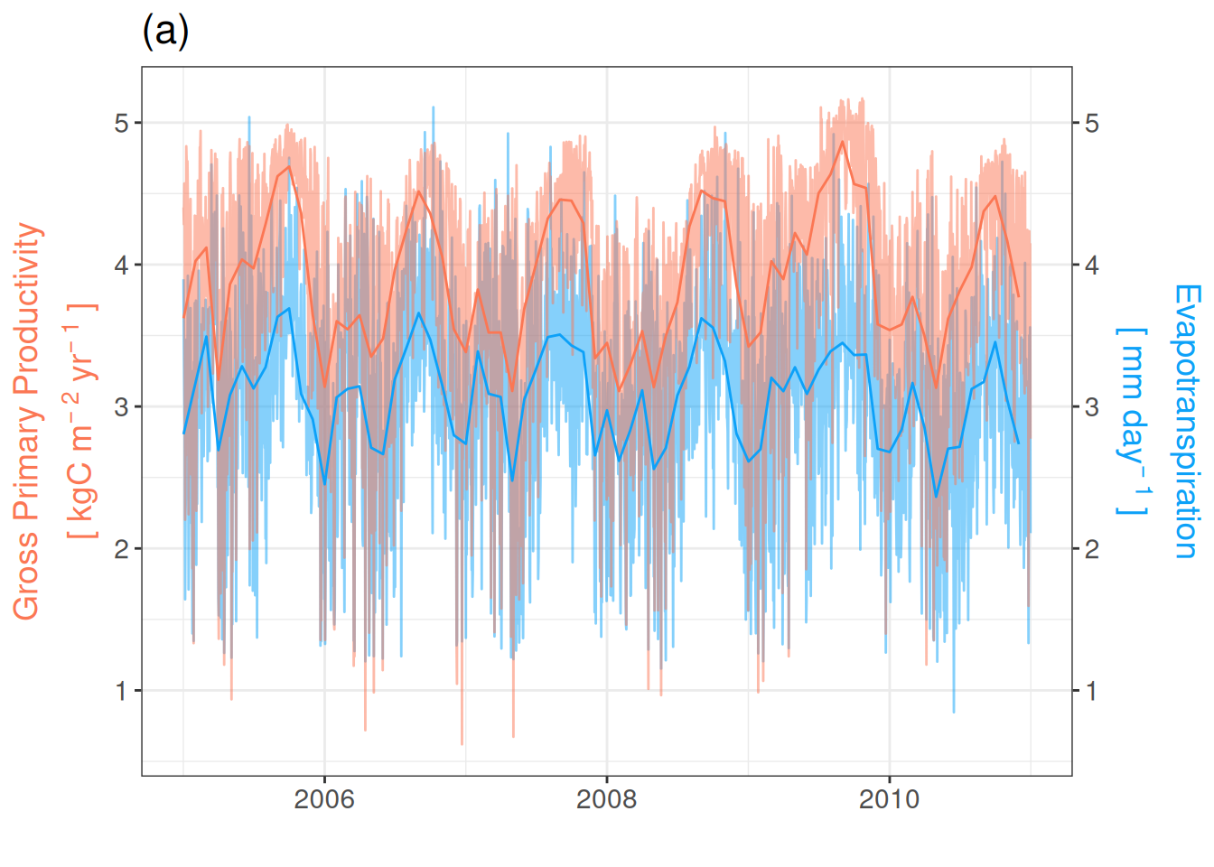
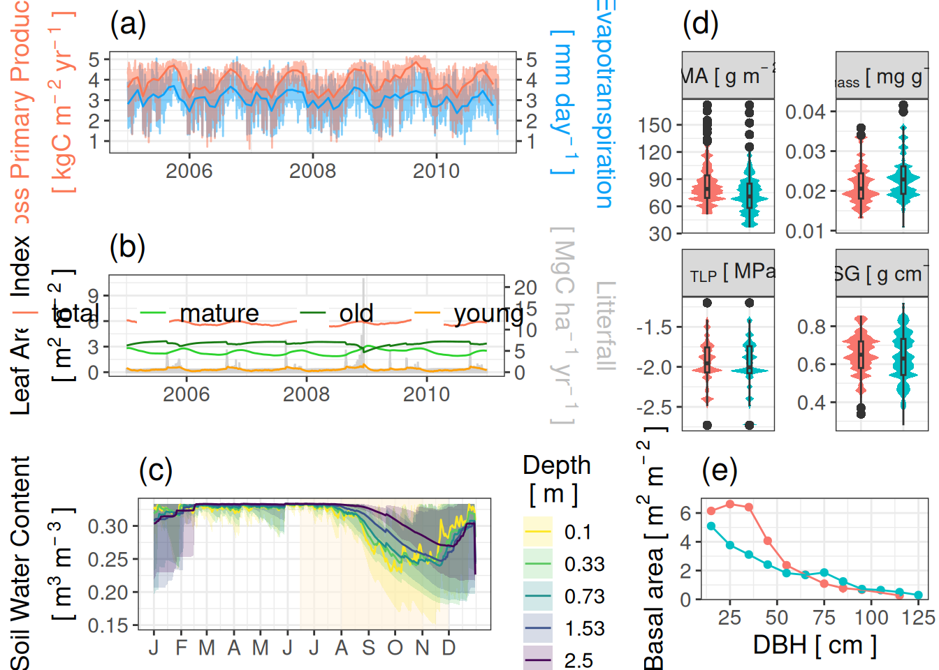
Daily and monthly means of growth primary productivity and evapotranspitation for Paracou. Dark lines are the monthly means, semi-transparent lines are the daily means variations.

Leaf area index & litterfall

Code

cols <- c("total" = "#fb7754", "young" = "#2bd22c", "mature" = "#197b14", "old" = "#ffa006")
lai <- read_tsv("outputs/evaluation_fluxes.tsv") %>% 
  filter(grepl("lai", variable)) %>% 
  filter(year(date) %in% 2005:2010) %>% 
  filter(site == "Paracou")
litter <- read_tsv("outputs/evaluation_fluxes.tsv") %>% 
  filter(variable == "litter") %>% 
  filter(year(date) %in% 2005:2010) %>% 
  mutate(simulated = simulated/2) %>% 
  filter(site == "Paracou")
gb <- lai %>% 
  ggplot(aes(date, simulated, col = variable)) +
  geom_col(col = "lightgrey", data = litter) +
  geom_line() +
  theme_bw() +
  theme(legend.position = "bottom") +
  xlab("") +
  scale_color_manual(name = "", 
                     values = as.vector(cols), 
                     labels = c("total", "mature", "old", "young")) +
  scale_y_continuous(
    name = expression(atop("Leaf Area Index", 
                           "["~m^2~m^{-~2}~"]")),
    sec.axis = sec_axis(trans = ~.*2,
                        name = expression(atop("Litterfall",
                                               "["~MgC~ha^{-~1}~yr^{-~1}~"]")))
  ) +
  guides(colour = guide_legend(nrow = 1)) +
    theme(
    axis.title.y = element_text(color = "black"),
    axis.title.y.right = element_text(color = "grey"),
    legend.position = c(0.4, 0.8),
    legend.background = element_rect(colour = NA, fill = NA),
    text = element_text(size = text_size),
    legend.text = element_text(size = text_size),
    legend.key.spacing.x = unit(20, "pt")
  ) +
  ggtitle("(b)")
gb

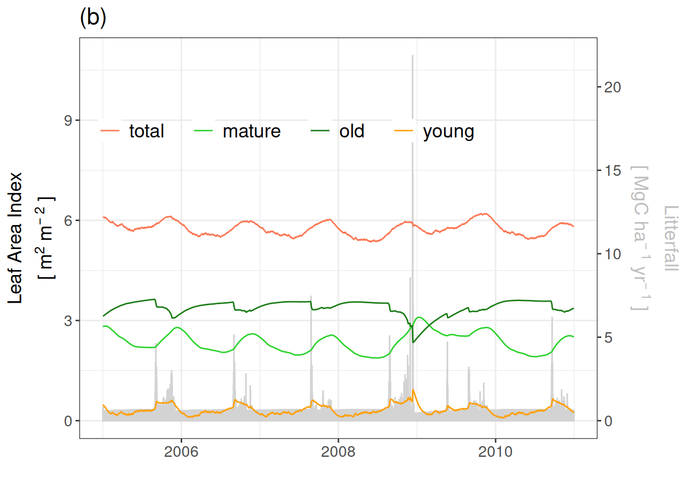
Daily means of leaf area index and litterfall for Paracou with leaf cohorts of total, yound, mature and old leaves indicated with coloured lines and litterfall with grey bars.

Soil water content

Code

gc <- read_tsv("outputs/evaluation_fluxes.tsv") %>% 
   filter(grepl("^swc", variable)) %>% 
  mutate(depth = as.numeric(gsub("swc", "", variable))) %>% 
  mutate(depth = recode(paste(site, depth), 
                        "Paracou 0" = 0.1,
                        "Tapajos 0" = 0.1,
                        "Paracou 1" = 0.33,
                        "Tapajos 1" = 0.5,
                        "Paracou 2" = 0.73,
                        "Tapajos 2" = 1.5,
                        "Paracou 3" = 1.53,
                        "Tapajos 3" = 4,
                        "Paracou 4" = 2.5,
                        "Tapajos 4" = 16.1)) %>% 
  group_by(site, depth, day = yday(date)) %>% 
  summarise(l = quantile(simulated, 0.025, na.rm = TRUE), 
            m = mean(simulated, na.rm = TRUE), 
            h = quantile(simulated, 0.975, na.rm = TRUE)) %>% 
  mutate(depth = as.factor(depth)) %>% 
  filter(site == "Paracou") %>% 
  ggplot(aes(day, m)) +
  geom_rect(aes(xmin = day, xmax = end), fill  = "#fff4e0",
           ymin = -Inf, ymax = Inf, alpha = 0.5,
           data = data.frame(day = yday(as_date(c("2000-8-1", "2000-06-15"))),
                             m = -Inf,
                             end = yday(as_date(c("2000-12-1", "2000-11-1"))),
                             site = c("Paracou", "Tapajos"))) +
  geom_ribbon(aes(ymin = l, ymax = h, col = depth, fill = depth, group = depth),
              col = NA, alpha = 0.2) +
  geom_line(aes(col = depth, fill = depth, group = depth)) +
  theme_bw() +
  scale_color_viridis_d("Depth\n [ m ]", direction = -1) +
  scale_fill_viridis_d("Depth\n [ m ]", direction = -1) +
  theme(axis.title.x = element_blank(),
        text = element_text(size = text_size)) +
  ylab(expression(atop("Soil Water Content", 
                       "["~m^{3}~m^{-~3}~"]"))) +
  scale_x_continuous(breaks = c(1, 32, 61, 92, 122, 153, 183, 214, 245, 275, 306, 336),
                    labels = c("J", "F", "M", "A", "M", "J", "J", "A", "S", "O", "N", "D"))+
  ggtitle("(c)")
gc

Mean annual cycle of daily means of soil water content at Paracou and Tapajos across ten years and for 5 differents depths.

Forest structure

Code

ge <- read_tsv("outputs/evaluation_forest.tsv") %>% 
  mutate(plot = repetition) %>% 
  select(site, plot, dbh) %>% 
  mutate(dbh_class = cut(dbh, breaks = seq(10, 200, by = 10), 
                         labels = seq(10, 190, by = 10)+5)) %>% 
  mutate(dbh_class = as.numeric(as.character(dbh_class))) %>% 
  group_by(site, plot, dbh_class) %>% 
  summarise(abundance = n()/4,
            ba = sum((dbh/2)^2*pi)/10^4/4) %>% 
  mutate(log_abundance = log10(abundance)) %>% 
  gather(variable, simulated, -site, -dbh_class, -plot) %>% 
  gather(type, value, -site, -dbh_class, -variable, -plot) %>% 
  group_by(site, dbh_class, variable, type) %>% 
  summarise(l = quantile(value, 0.025, na.rm = TRUE), 
            m = quantile(value, 0.5, na.rm = TRUE), 
            h = quantile(value, 0.975, na.rm = TRUE)) %>% 
  na.omit() %>% 
  filter(variable == "ba") %>% 
  ggplot(aes(dbh_class, m, col = site, group = site)) +
  geom_linerange(aes(ymin = l, ymax = h)) +
  geom_point() +
  geom_line() +
  theme_bw() +
  xlab("DBH [ cm ]") + 
  ylab(expression(Basal~area~"["~m^{2}~m^{-~2}~"]")) +
  theme(legend.position = "bottom",
        text = element_text(size = text_size)) +
  scale_color_discrete("", guide = "none") +
  ggtitle("(e)")
ge

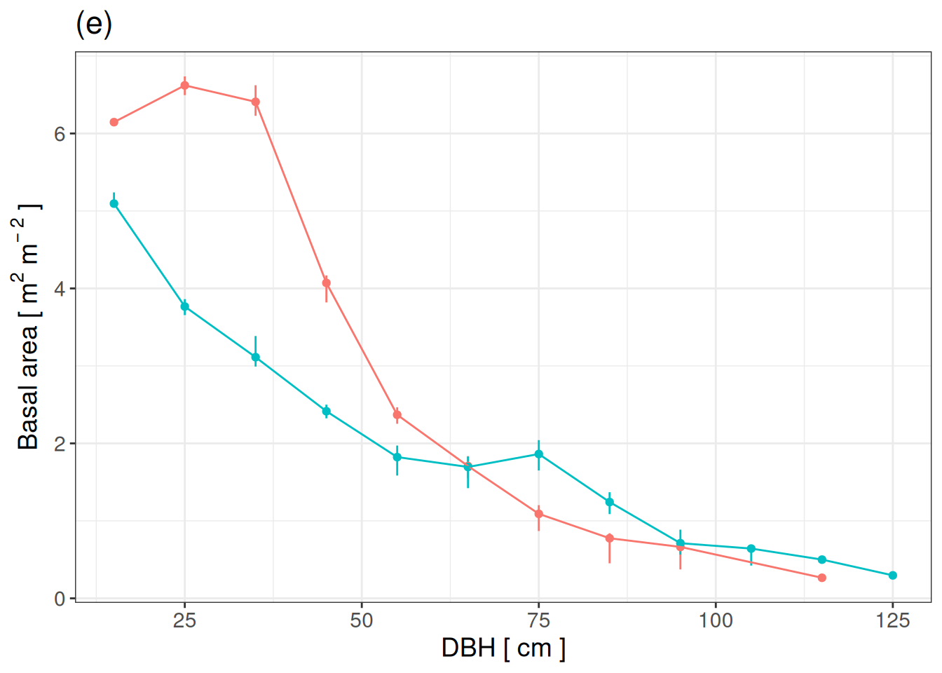
Evaluation of the size structure estimated by TROLL at the Paracou and Tapajos sites, expressed in terms of basal area. The confidence on the TROLL values was estimated generating an ensemble of 10 simulations (see methods).

Functional traits

Code

troll_traits <- list(
    read_tsv("outputs/Paracou_species_troll.tsv"),
    read_tsv("outputs/Tapajos_species_troll.tsv")
) %>% bind_rows() %>% 
  unique() %>% 
  rename_all(~ gsub("s_", "", .)) %>% 
  select(-seedmass, -regionalfreq) %>% 
  rename(species = name) %>% 
  mutate(species = gsub("_", " ", species)) %>% 
  gather(trait, trait_value, -species)
troll_traitdist <- read_tsv("outputs/evaluation_forest.tsv") %>% 
  mutate(plot = repetition) %>% 
  select(site, plot, species) %>% 
  left_join(troll_traits) %>% 
  filter(trait %in% c("LMA", "Nmass", "tlp", "wsg")) %>% 
  mutate(traitlong = recode(trait, 
                            "ah" = 'a[h]~"["~m~"]"',
                            "dbhmax" = 'dbh[max]~"["~m~"]"',
                            "hmax" = 'h[max]~"["~m~"]"',
                            "leafaera" = 'LA~"["~cm^{2}~"]"',
                            "LMA" = 'LMA~"["~g~m^{-~2}~"]"',
                            "Nmass" = 'N[mass]~"["~mg~g^{-~1}~"]"',
                            "Pmass" = 'P[mass]~"["~mg~g^{-~1}~"]"',
                            "tlp" = 'pi[~" TLP"]~"["~MPa~"]"',
                            "wsg" = 'WSG~"["~g~cm^{-~3}~"]"'))
gd <- troll_traitdist %>% 
  ggplot(aes(site, trait_value, fill = site)) +
  geom_violin(col = NA) +
  geom_boxplot(width=0.1) +
  facet_wrap(~ traitlong, scales = "free", labeller = label_parsed) +
  theme_bw() +
  scale_fill_discrete("", guide = "none") +
  theme(axis.title = element_blank(), axis.text.x = element_blank(),
        axis.ticks.x = element_blank(), legend.position = "bottom",
        text = element_text(size = text_size)) +
  ggtitle("(d)")
gd

Functional composition estimated by TROLL at the Paracou and Tapajos site expressed in terms of distribution per trait and site.

Assembly

Code

g <- gridExtra::grid.arrange(ga, gb, gc, gd, ge,
                        layout_matrix = rbind(c(1, 1, 4),
                                              c(2, 2, 4),
                                              c(3, 3, 5)))

Code

ggsave("figures/companion_f01.png", g, dpi = 300, width = 16, height = 10, bg = "white")