Calibration of forest structure parameters (crown radius allometry and mortality) in TROLL 3.1.8:
\(m\) : minimal death rate in death per year calibrated to 0.025 at Nouragues
\(a_{CR}\) : crown radius intercept calibrated to 2.13 at Nouragues
\(b_{CR}\) : crown radius slope calibrated to 0.63 at Nouragues
Crown radius parameters variation
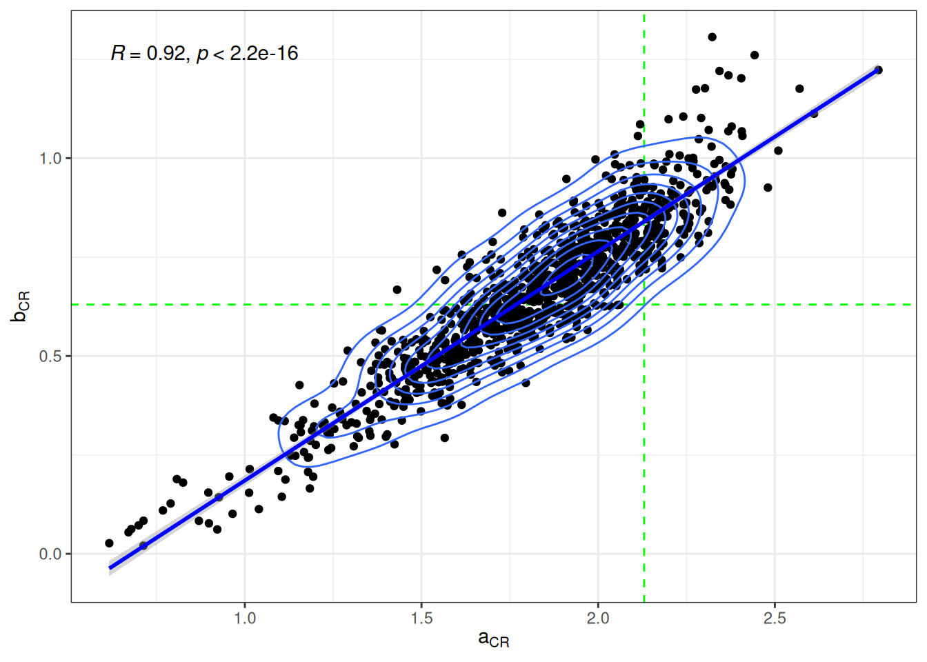
We gathered all Tallo measurements of crown radius and diameter in a radius of 10-km of Tapajos for trees above 10-cm. We randomly selected 10 trees per class diameter of decimetre a thousand times and computed crown radius intercepts and slopes. We obtained a parameter distribution with a correlation of 0.91, a linear regression of \(b_{CR} = -0.39+0.57 \times a_{CR}\), and a standard variation of 0.08. Dashed lines shows Paracou values, which are lower than the observations.
Code
tapajos <-tibble(site =c("Tapajos"),latitude =c(-2.85667),longitude =c(-54.9588900),) %>%st_as_sf(coords =c("longitude", "latitude"), crs =4326) %>%st_buffer(10^4)params <-read_csv("data/species/tallo.csv") %>%filter(longitude <=-39, longitude >=-79, latitude >=-18, latitude <=10) %>%st_as_sf(coords =c("longitude", "latitude"), crs =4326) %>%st_intersection(tapajos) %>%filter(!is.na(crown_radius_m), !is.na(stem_diameter_cm)) %>%mutate(dbh_m = stem_diameter_cm *0.01) %>%filter(dbh_m >=0.1) %>%mutate(class_dbh_dm =floor(dbh_m *10)) %>%mutate(rep =list(1:10^3)) %>%unnest(rep) %>%group_by(rep) %>%sample_n(10, replace = T) %>%unique() %>%st_drop_geometry() %>%ungroup() %>%nest_by(rep) %>%mutate(coefs =list(coef(lm(log(crown_radius_m) ~log(dbh_m), data = data)))) %>%mutate(a = coefs[1], b = coefs[2]) %>%select(rep, a, b) %>%filter(a >0, b >0)
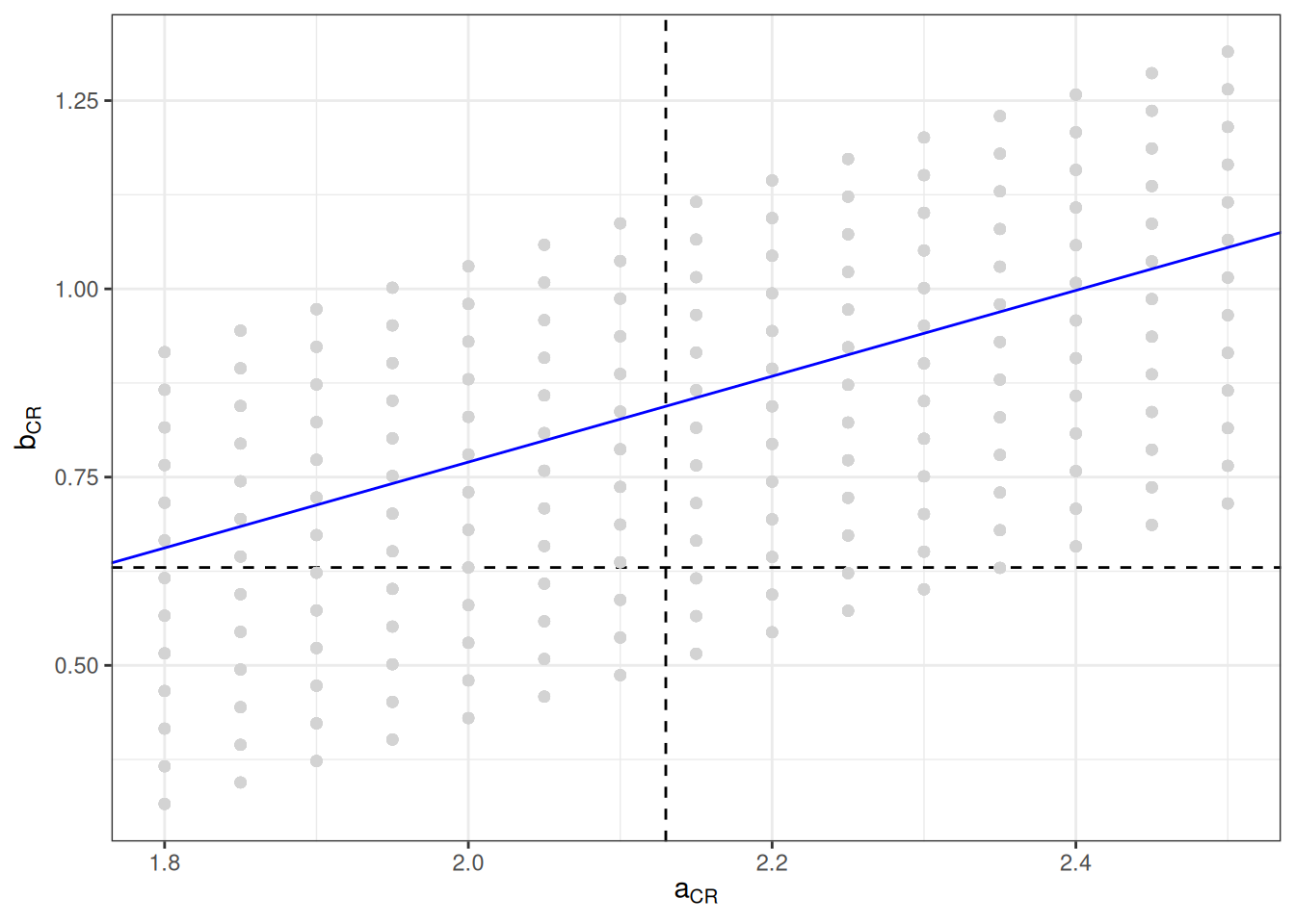
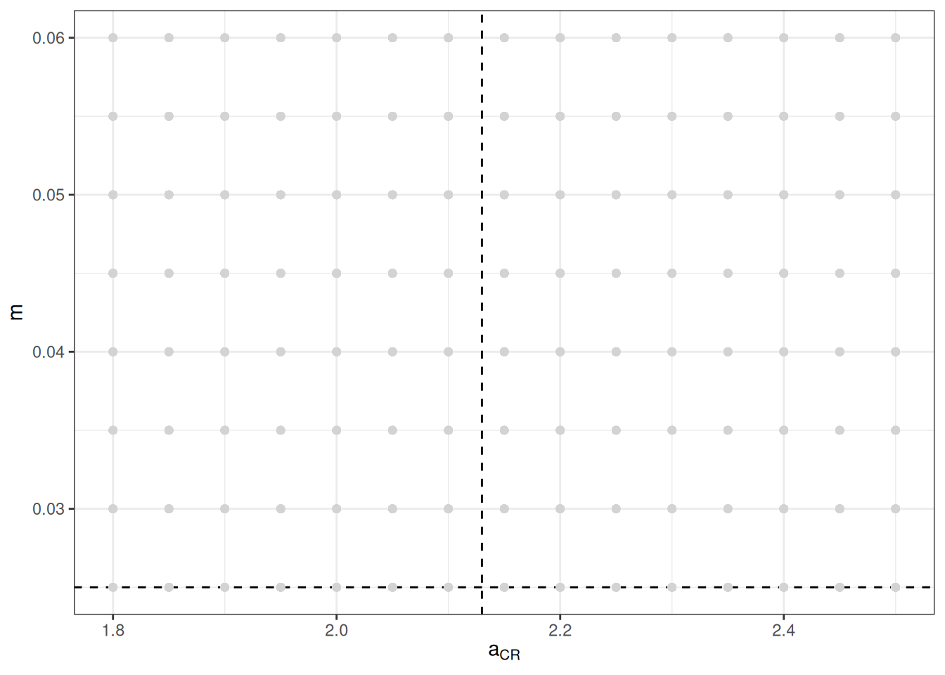
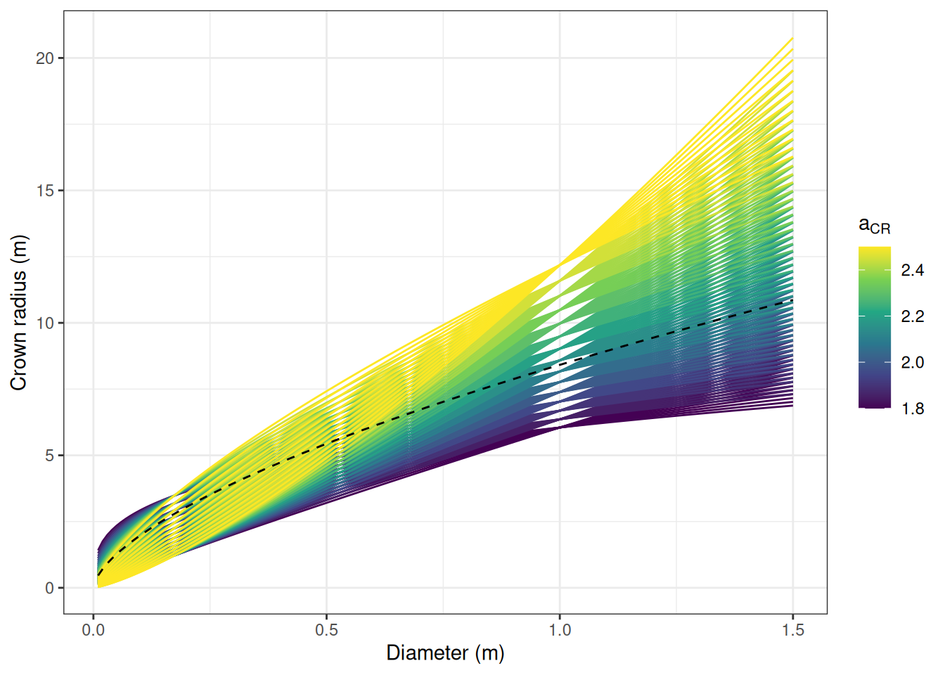
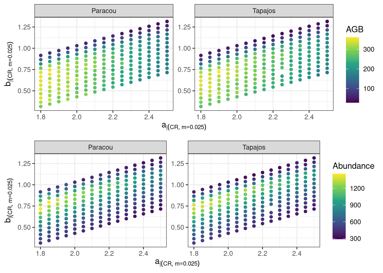
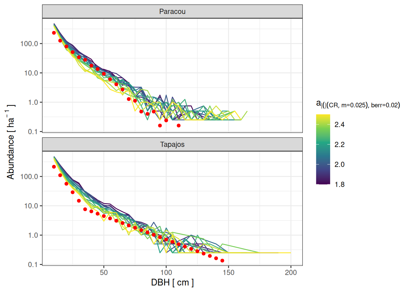
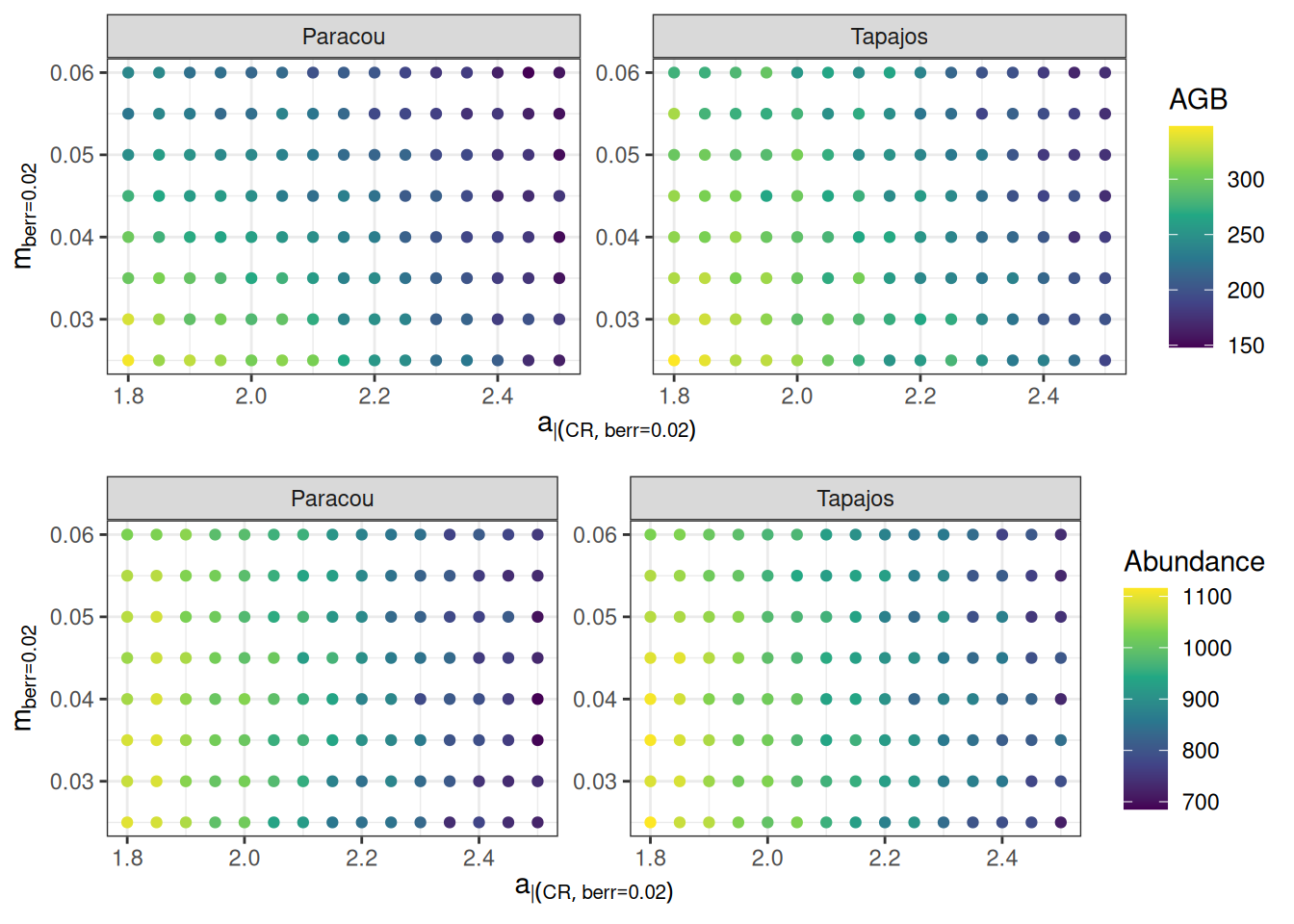
We prepared the parameter space for calibration defining low limit, high limit, and step for a, m, and the error of b. b was computed using the linear equation plus the error. We used \(3 \sigma\) for the error. We obtained a calibration grid of 11,193 simulations. Dashed lines shows Paracou values which are thus lower. The last figure shows the corresponding projected allometries of crown radius.
Code
pars <-data.frame(parameter =c("a", "error_b", "m"),low =c(1.8, -4*0.08, 0.025),high =c(2.5, 4*0.08, 0.06),by =c(0.05, 0.05, 0.005))grid <-data.frame(a =seq(pars$low[1], pars$high[1], by = pars$by[1])) %>%mutate(error_b =list(seq(pars$low[2], pars$high[2], by = pars$by[2]))) %>%unnest(error_b) %>%mutate(b =-0.39+0.57*a + error_b) %>%mutate(m =list(seq(pars$low[3], pars$high[3], by = pars$by[3]))) %>%unnest(m)
dat <-read_tsv("outputs/calib_structure.tsv") %>%group_by(site, a, b, m) %>%summarise(agb =sum(agb)/10^3/2,abundance =sum(abundance)) %>%mutate(berr =-0.39+0.57*a - b) %>%filter(berr >0, berr <0.05)cowplot::plot_grid( dat %>%ggplot(aes(a, m, col = agb)) +geom_point() +facet_wrap(~ site, scales ="free_y") +theme_bw() +scale_color_viridis_c("AGB") +xlab(expression(a[CR|berr==0.02])) +ylab(expression(m[berr==0.02])), dat %>%ggplot(aes(a, m, col = abundance)) +geom_point() +facet_wrap(~ site, scales ="free_y") +theme_bw() +scale_color_viridis_c("Abundance") +xlab(expression(a[CR|berr==0.02])) +ylab(expression(m[berr==0.02])),nrow =2)
Code
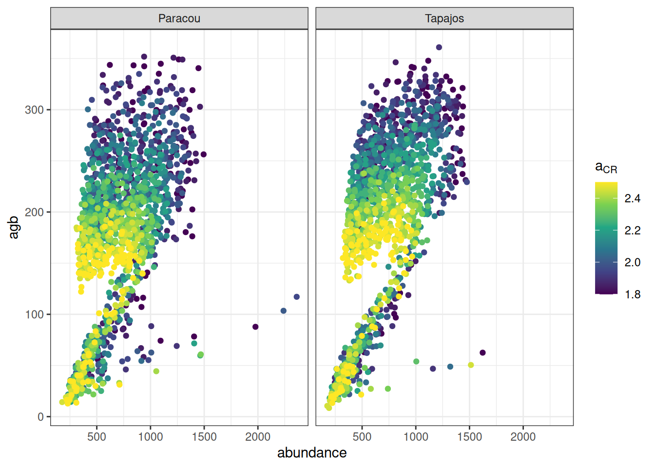
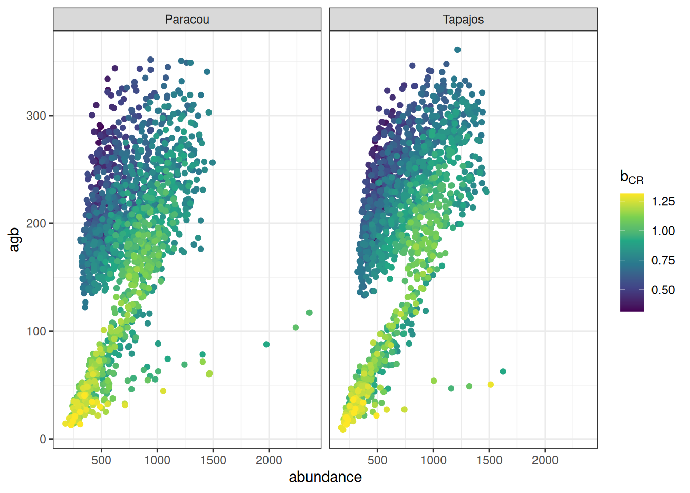
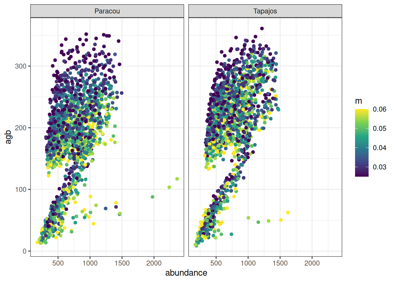
read_tsv("outputs/calib_structure.tsv") %>%group_by(site, a, b, m) %>%summarise(abundance =sum(abundance), agb =sum(agb)/10^3/2) %>%ggplot(aes(abundance, agb, col = m)) +geom_point() +theme_bw() +scale_color_viridis_c(expression(m)) +facet_wrap(~ site)
Code
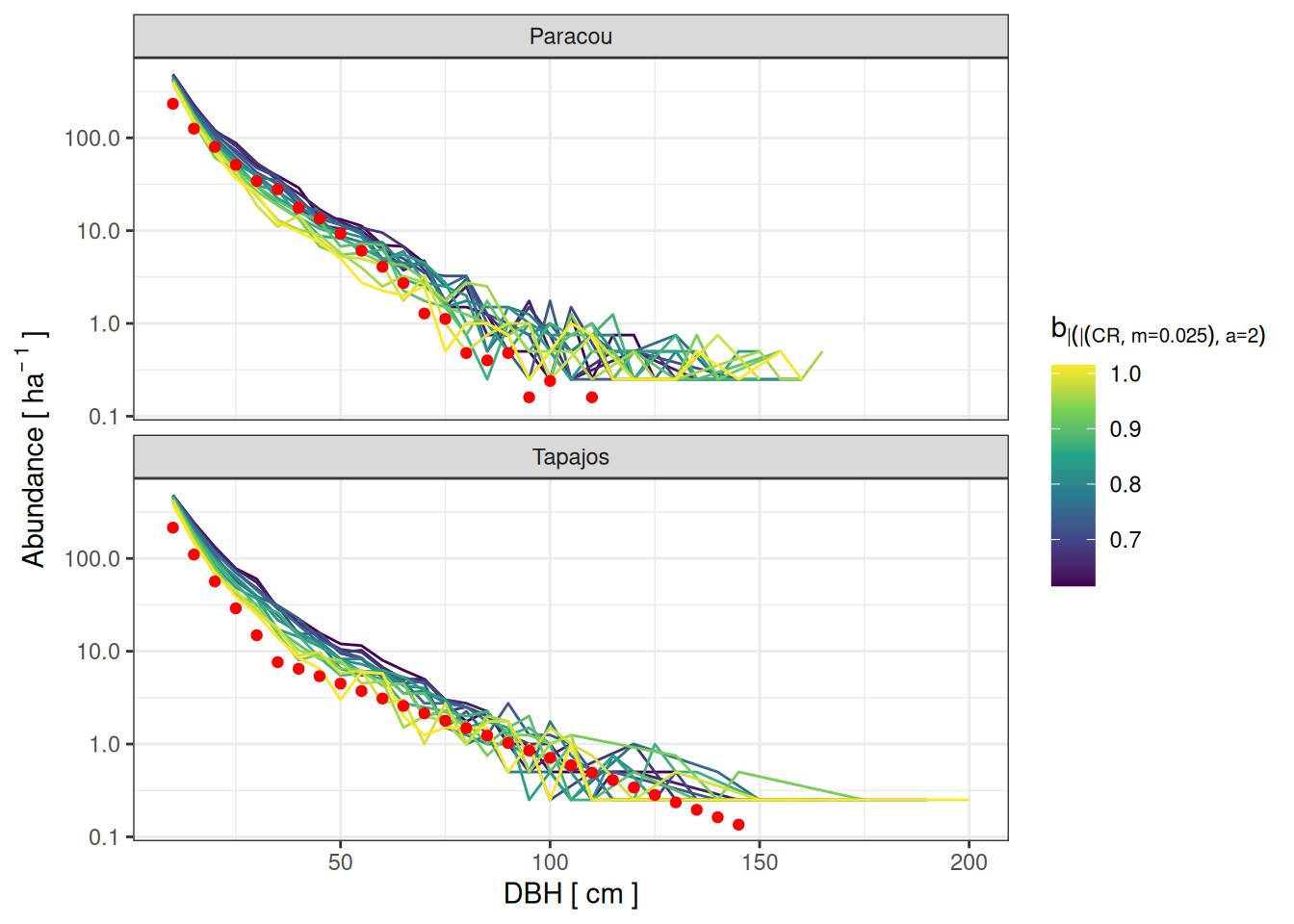
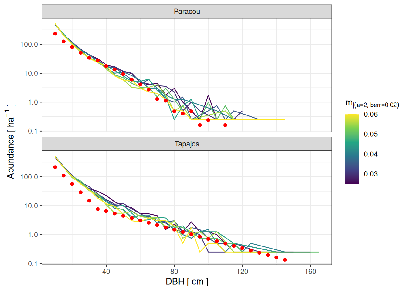
read_tsv("outputs/calib_structure.tsv") %>%filter(a ==2) %>%mutate(berr =-0.39+0.57*a - b) %>%filter(berr >0, berr <0.05) %>%ggplot(aes(dbh_class, abundance)) +geom_line(aes(col = m, group =paste(a, b, m))) +geom_point(data =filter(obs, dbh_class <150), col ="red") +scale_y_log10(labels = scales::comma) +xlab("DBH [ cm ]") +ylab(expression(Abundance~"["~ha^{-~1}~"]")) +scale_color_viridis_c(expression(m)) +scale_color_viridis_c(expression(m[a==2|berr==0.02])) +theme_bw() +facet_wrap(~ site, nrow =2)
Rice, Amy H., Elizabeth Hammond Pyle, Scott R. Saleska, Lucy Hutyra, Michael Palace, Michael Keller, Plínio B. de Camargo, Kleber Portilho, Dulcyana F. Marques, and Steven C. Wofsy. 2004. “CARBON BALANCE AND VEGETATION DYNAMICS IN AN OLD-GROWTH AMAZONIAN FOREST.”Ecological Applications 14 (sp4): 55–71. https://doi.org/10.1890/02-6006.
Rutishauser, Ervan, Fabien Wagner, Bruno Herault, Eric-André Nicolini, and Lilian Blanc. 2010. “Contrasting Above-Ground Biomass Balance in a Neotropical Rain Forest.”Journal of Vegetation Science, March. https://doi.org/10.1111/j.1654-1103.2010.01175.x.